library(ggplot2)
library(dplyr)

te <- list(ink="#16241d", body="#2c3a31", forest="#275139", label="#46604a",
           sage="#93a87f", paper="#f5f4ee", line="#dad9ca", faint="#5d6b61", rust="#b5534e")
theme_te <- function(base_size = 11) {
  theme_minimal(base_size = base_size) +
    theme(text = element_text(colour = te$body),
          plot.title = element_text(colour = te$ink, face = "bold", size = rel(1.02)),
          plot.subtitle = element_text(colour = te$faint, size = rel(0.9)),
          axis.title = element_text(colour = te$label),
          axis.text = element_text(colour = te$faint),
          panel.grid.major = element_line(colour = te$line, linewidth = 0.3),
          panel.grid.minor = element_blank(),
          panel.background = element_rect(fill = te$paper, colour = NA),
          plot.background = element_rect(fill = te$paper, colour = NA),
          legend.key = element_rect(fill = te$paper, colour = NA),
          strip.text = element_text(colour = te$forest, face = "bold"))
}

pars <- list(a_s=-1.4, b_s=0.50, a_g=1.9, b_g=0.65, sig_g=0.90,
a_f=-6.0, b_f=0.80, a_r=0.42, b_r=0.24, mu_r=2.2, sig_r=0.70)IPM sensitivity and elasticity
population dynamics
demography
integral projection models
R
ecology tutorial
Sensitivity and elasticity of an integral projection kernel in R: the continuous analogue of matrix perturbation analysis, split between survival and fecundity.
Once you have a kernel and its growth rate lambda (see building an integral projection model), the next question is which parts of the life cycle matter most. For a matrix model this is sensitivity and elasticity analysis; for an integral projection model the same idea becomes a surface over parent size and offspring size. Sensitivity asks how lambda responds to a small absolute change in the kernel at each size pair; elasticity rescales that to a proportional change and sums to one, which lets you split lambda’s sensitivity cleanly between survival and reproduction. The mechanics carry over from the matrix case, with one continuous-model wrinkle around the boundary.
The kernel and its two eigenvectors
Build the eviction-corrected kernel on bounds that cover the size range, keeping its survival-growth and fecundity parts separate for the decomposition later. Perturbation analysis needs both eigenvectors: the dominant right eigenvector is the stable size distribution w(z), and the dominant left eigenvector is the reproductive value v(z).
build_K <- function(L, U, m) {
  h    <- (U - L) / m
  mesh <- L + (1:m - 0.5) * h
  S  <- plogis(pars$a_s + pars$b_s * mesh)
  G  <- outer(mesh, mesh, function(zp, z) dnorm(zp, pars$a_g + pars$b_g * z, pars$sig_g))
  G  <- sweep(G, 2, colSums(G) * h, "/")
  Cr <- dnorm(mesh, pars$mu_r, pars$sig_r); Cr <- Cr / (sum(Cr) * h)
  P  <- sweep(G, 2, S, "*") * h
  Pf <- plogis(pars$a_f + pars$b_f * mesh); Rn <- exp(pars$a_r + pars$b_r * mesh)
  Fk <- outer(Cr, Pf * Rn) * h
  list(K = P + Fk, P = P, Fk = Fk, mesh = mesh, h = h)
}

L <- 0; U <- 14; m <- 100
k <- build_K(L, U, m); K <- k$K; mesh <- k$mesh; h <- k$h

ev  <- eigen(K); lambda <- Re(ev$values[1])
w   <- Re(ev$vectors[, 1]); if (w[which.max(abs(w))] < 0) w <- -w; w <- w / sum(w)
v   <- Re(eigen(t(K))$vectors[, 1]); if (v[which.max(abs(v))] < 0) v <- -v
v   <- v / v[which.max(w)]                 # reproductive value scaled to 1 at the modal size
lambda
[1] 1.013295Sensitivity: a surface over size pairs
The sensitivity of lambda to the kernel at the size pair (z’, z) is
s(z’, z) = v(z’) w(z) / <v, w>,
the outer product of reproductive value and the stable distribution, divided by their inner product. This is the exact analogue of the matrix formula S_ij = v_i w_j / (v . w); on the mesh you build it from the eigenvectors and divide by the bin width to recover the kernel function rather than the matrix entry. A finite-difference check confirms it: nudge one matrix entry and the change in lambda matches the analytic value.
Smat <- outer(v, w) / sum(v * w)           # sensitivity of matrix entries: dlambda/dK_ij
Sfun <- Smat / h                           # kernel sensitivity function s(z', z)

i0 <- which.min(abs(mesh - 3)); j0 <- which.min(abs(mesh - 8))
delta <- 1e-6; Kp <- K; Kp[i0, j0] <- Kp[i0, j0] + delta
c(numerical = (Re(eigen(Kp)$values[1]) - lambda) / delta, analytic = Smat[i0, j0])
numerical analytic
0.0004683944 0.0004683964 idx <- which(Sfun == max(Sfun), arr.ind = TRUE)
zmax_from <- mesh[idx[2]]; zmax_to <- mesh[idx[1]]; Kval_there <- K[idx[1], idx[2]]
long <- function(M) data.frame(z = rep(mesh, each = m), zp = rep(mesh, times = m), val = as.vector(M))
ggplot(long(Sfun), aes(z, zp, fill = val)) +
geom_raster(interpolate = TRUE) +
scale_fill_gradient(low = te$paper, high = te$forest, name = "sensitivity") +
annotate("point", x = zmax_from, y = zmax_to, colour = te$rust, size = 2.2) +
coord_equal(expand = FALSE) +
labs(x = "Size z at time t (parent)", y = "Size z' at time t+1 (offspring or survivor)") +
theme_te(11) + theme(panel.grid = element_blank())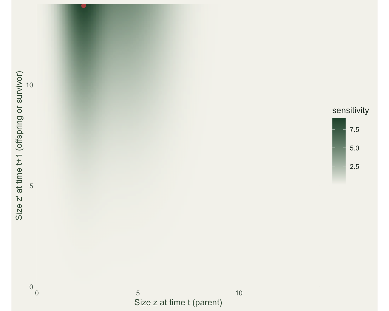
The finite-difference and analytic sensitivities agree to nine decimals. The surface makes a point that trips up management readers: sensitivity is largest at parent size 2.3 producing offspring size 13.9, the upper-left corner, where the kernel itself is about 5e-32. Sensitivity does not care whether a transition is biologically possible; it asks only what lambda would do if that pathway existed. That makes it the right currency for an evolutionary question (which new phenotype would help) and the wrong one for a manager choosing among things they can actually change. This is the continuous version of a matrix sensitivity peaking on a structural zero.
Elasticity: proportional change, and where it lives
Elasticity fixes that by weighting sensitivity with the kernel value:
e(z’, z) = (K(z’, z) / lambda) s(z’, z).
Because it is scaled by the kernel, elasticity is zero wherever the kernel is zero, and it sums to one across the surface. That normalisation is what makes the survival-versus-reproduction split meaningful.
E   <- (K / lambda) * Smat                 # elasticity of matrix entries; sums to 1
e_P <- sum((k$P  / lambda) * Smat)         # survival-growth elasticity
e_F <- sum((k$Fk / lambda) * Smat)         # fecundity elasticity
c(total = sum(E), survival_growth = e_P, fecundity = e_F)
total survival_growth fecundity
1.0000000 0.8502407 0.1497593 ggplot(long(E), aes(z, zp, fill = val)) +
geom_raster(interpolate = TRUE) +
geom_abline(slope = 1, intercept = 0, linetype = "dashed", colour = "#ffffffaa", linewidth = 0.4) +
scale_fill_gradient(low = te$paper, high = te$forest, trans = "sqrt", name = "elasticity") +
coord_equal(expand = FALSE) +
labs(x = "Size z at time t", y = "Size z' at time t+1") +
theme_te(11) + theme(panel.grid = element_blank())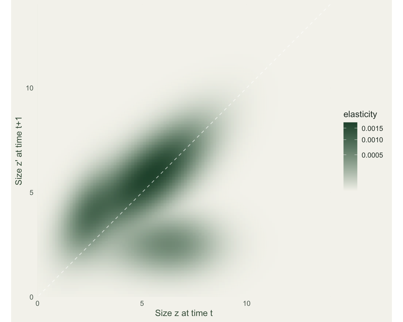
The elasticities sum to 1, as they must. Splitting them by process, survival and growth account for 85 per cent of lambda’s proportional sensitivity and fecundity for only 15 per cent. For this long-lived plant, holding existing individuals in the population (and moving them up in size) does far more for lambda than adding recruits. That is the same conclusion the classic loggerhead turtle analysis reached: protecting large juveniles and adults outperforms protecting eggs, because lambda is proportionally far more elastic to adult survival than to fecundity, however many eggs a female lays.
Takeaway
Sensitivity and elasticity move from matrix to kernel almost unchanged: the eigenvectors become eigenfunctions, the outer product becomes a surface, and the finite-difference check still works. Sensitivity tells you the shape of selection, including on transitions that cannot happen; elasticity tells you where proportional management effort pays off, and its survival-versus-fecundity split turns a kernel into a conservation recommendation.
References
Easterling MR, Ellner SP, Dixon PM 2000. Ecology 81(3):694-708 (10.1890/0012-9658(2000)081[0694:SSSAAN]2.0.CO;2).
Ellner SP, Rees M 2006. American Naturalist 167(3):410-428 (10.1086/499438).
de Kroon H, Plaisier A, van Groenendael J, Caswell H 1986. Ecology 67(5):1427-1431 (10.2307/1938700).
Crouse DT, Crowder LB, Caswell H 1987. Ecology 68(5):1412-1423 (10.2307/1939225).
Merow C, Dahlgren JP, Metcalf CJE, Childs DZ, Evans MEK, Jongejans E, Record S, Rees M, Salguero-Gomez R, McMahon SM 2014. Methods in Ecology and Evolution 5(2):99-110 (10.1111/2041-210X.12146).
Caswell H 2001. Matrix Population Models. 2nd ed. Sinauer Associates. ISBN 978-0-87893-096-8.