library(ggplot2)
library(dplyr)

te <- list(ink="#16241d", body="#2c3a31", forest="#275139", label="#46604a",
           sage="#93a87f", paper="#f5f4ee", line="#dad9ca", faint="#5d6b61", rust="#b5534e")
theme_te <- function(base_size = 11) {
  theme_minimal(base_size = base_size) +
    theme(text = element_text(colour = te$body),
          plot.title = element_text(colour = te$ink, face = "bold", size = rel(1.02)),
          plot.subtitle = element_text(colour = te$faint, size = rel(0.9)),
          axis.title = element_text(colour = te$label),
          axis.text = element_text(colour = te$faint),
          panel.grid.major = element_line(colour = te$line, linewidth = 0.3),
          panel.grid.minor = element_blank(),
          panel.background = element_rect(fill = te$paper, colour = NA),
          plot.background = element_rect(fill = te$paper, colour = NA),
          legend.key = element_rect(fill = te$paper, colour = NA),
          strip.text = element_text(colour = te$forest, face = "bold"))
}

pars <- list(a_s=-1.4, b_s=0.50, a_g=1.9, b_g=0.65, sig_g=0.90,
a_f=-6.0, b_f=0.80, a_r=0.42, b_r=0.24, mu_r=2.2, sig_r=0.70)Eviction and mesh size in an IPM
population dynamics
demography
integral projection models
R
ecology tutorial
Two numerical traps in integral projection models: eviction of mass off the size boundary, and mesh size. See how each biases lambda in R, and how to fix them.
An integral projection model looks continuous, but the moment you take its dominant eigenvalue you are working with a matrix: the midpoint rule (see building an integral projection model) evaluates the kernel on a grid and multiplies by the bin width. That discretisation carries two failure modes that quietly bias the growth rate lambda. The first is eviction: a Gaussian growth density on a bounded size range loses probability mass off the edges, so individuals vanish. The second is mesh size: too few bins under-resolve the kernel. Both push lambda in a predictable direction, and both are easy to check. This post uses a fixed, known kernel (no estimation) so that any movement in lambda is purely numerical.
A kernel builder that can correct eviction
The builder takes the size range [L, U] and the mesh size m, and has a switch for the eviction fix. The fix is a renormalisation: each growth column should integrate to one over all possible next-sizes, and if it integrates to less (because mass fell off the boundary), dividing by the realised integral reassigns that lost mass proportionally to the sizes that remain. The recruit-size density is treated the same way.
build_K <- function(L, U, m, correct = FALSE) {
  h    <- (U - L) / m
  mesh <- L + (1:m - 0.5) * h
  S  <- plogis(pars$a_s + pars$b_s * mesh)
  G  <- outer(mesh, mesh, function(zp, z) dnorm(zp, pars$a_g + pars$b_g * z, pars$sig_g))
  Cr <- dnorm(mesh, pars$mu_r, pars$sig_r)
  if (correct) {
    G  <- sweep(G, 2, colSums(G) * h, "/")   # each growth column integrates to 1
    Cr <- Cr / (sum(Cr) * h)                 # recruit-size density integrates to 1
  }
  P  <- sweep(G, 2, S, "*") * h
  Pf <- plogis(pars$a_f + pars$b_f * mesh)
  Rn <- exp(pars$a_r + pars$b_r * mesh)
  Fk <- outer(Cr, Pf * Rn) * h
  list(K = P + Fk, mesh = mesh, h = h, S = S, retained = colSums(P))
}
Trap one: eviction at the boundary
Set the upper bound too close to the size of the largest plants and their growth spills over the edge. The survival-growth block then loses mass: the column sum of P falls below the survival probability s(z), which is exactly the fraction of survivors that should have gone somewhere. The gap is the evicted fraction.
m <- 100
tight  <- build_K(0, 8,  m, correct = FALSE)   # upper edge cuts off growth of large plants
tightc <- build_K(0, 8,  m, correct = TRUE)    # same bounds, eviction corrected
wide   <- build_K(0, 14, m, correct = FALSE)   # bounds cover the kernel; little is lost

lam_evict <- Re(eigen(tight$K)$values[1])
lam_corr  <- Re(eigen(tightc$K)$values[1])
lam_wide  <- Re(eigen(wide$K)$values[1])
c(evicting = lam_evict, corrected = lam_corr, wide_bounds = lam_wide)
evicting corrected wide_bounds
0.9951112 1.0029366 1.0131353 d1 <- data.frame(z = tight$mesh, frac = tight$retained / tight$S)
min_ret <- min(d1$frac); edge_z <- d1$z[which.min(d1$frac)]
ggplot(d1, aes(z, frac)) +
geom_hline(yintercept = 1, linetype = "dashed", colour = te$faint, linewidth = 0.4) +
geom_line(colour = te$forest, linewidth = 1) +
annotate("point", x = edge_z, y = min_ret, colour = te$rust, size = 2.4) +
scale_y_continuous(limits = c(0.8, 1.02)) +
labs(x = "Size z at time t", y = "Fraction of survival retained") +
theme_te(11)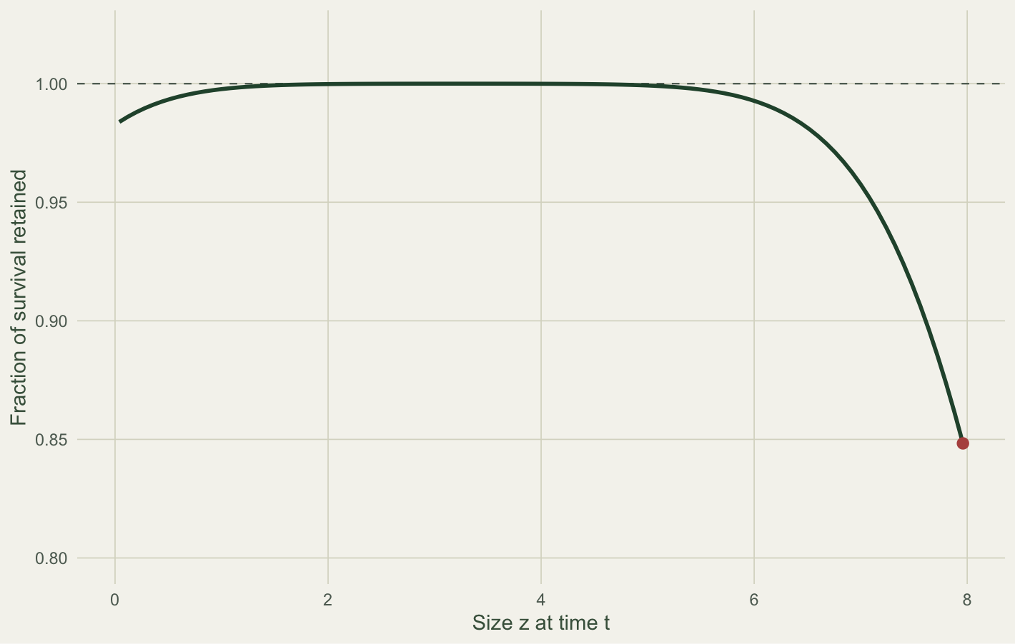
On these tight bounds the growth rate is lambda = 0.995. Renormalising lifts it to 1.003: that difference, 0.008, is the pure eviction effect, the mass that was silently discarded. The lowest retained fraction is 0.848 at size 7.96, right at the upper edge.
But notice the corrected value, 1.003, still falls short of the wide-bounds result, 1.013. That remaining gap is a different problem. Renormalisation conserves mass, but it cannot invent size classes that the domain excludes: bounds of 0 to 8 simply do not contain the large plants (which reach past 10 here), and those plants matter for lambda. Eviction and an inadequate domain are two separate mistakes. The correction handles the first; only wider bounds handle the second. In practice you want both: pad the range well beyond the observed sizes and keep the eviction correction on, at which point little mass is lost anyway.
Trap two: mesh size
With bounds that cover the kernel and the correction switched on, the only thing left to choose is m, the number of bins. The midpoint rule is an O(h^2) quadrature, so a coarse mesh under-resolves the sharp features (here the narrow recruit-size peak) and biases lambda low. Refining the mesh converges it.
ms    <- c(5, 10, 15, 20, 30, 50, 75, 100, 200, 500)
lam_m <- sapply(ms, function(mm) Re(eigen(build_K(0, 14, mm, correct = TRUE)$K)$values[1]))
lam_ref <- lam_m[length(lam_m)]
data.frame(m = ms, lambda = round(lam_m, 5), error = signif(lam_m - lam_ref, 2))
m lambda error
1 5 0.93454 -7.9e-02
2 10 1.01050 -2.8e-03
3 15 1.01323 -7.0e-05
4 20 1.01325 -4.5e-05
5 30 1.01327 -2.2e-05
6 50 1.01329 -8.2e-06
7 75 1.01329 -3.7e-06
8 100 1.01329 -2.0e-06
9 200 1.01330 -4.5e-07
10 500 1.01330 0.0e+00d2 <- data.frame(m = ms, lambda = lam_m)
ggplot(d2, aes(m, lambda)) +
geom_hline(yintercept = lam_ref, linetype = "dashed", colour = te$faint, linewidth = 0.4) +
geom_line(colour = te$sage, linewidth = 0.7) +
geom_point(colour = te$forest, size = 2.2) +
scale_x_log10(breaks = ms) +
labs(x = "Mesh size m (number of bins, log scale)", y = "Dominant eigenvalue lambda") +
theme_te(11)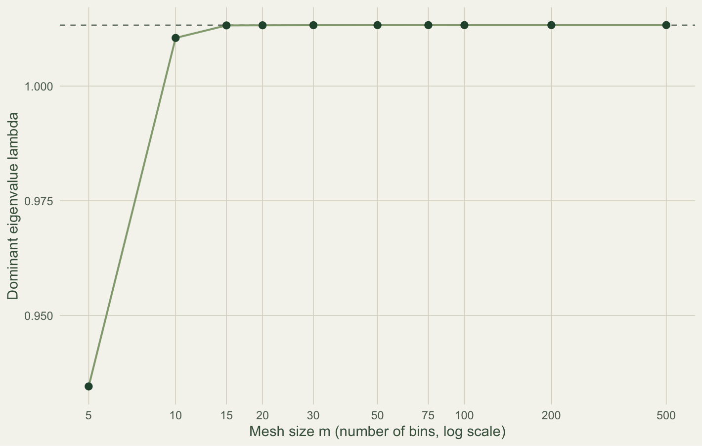
At m = 5 the estimate is lambda = 0.935, low by 7.8 per cent, because five bins cannot resolve a recruit distribution with a standard deviation of 0.7. By m = 20 the error is already under a ten-thousandth, and the value settles at 1.0133. For a kernel with narrow features you need a finer mesh than one with smooth ones; the safe move is to increase m until lambda stops changing to the precision you care about.
Practical checklist
Two habits remove both biases. Choose the size range with generous padding beyond the smallest and largest observed sizes, so the growth and recruit densities have room, and keep an eviction correction on so that whatever little mass still reaches the edge is conserved rather than discarded. Then confirm mesh convergence by doubling m and checking that lambda holds. Neither step is automatic in a hand-built kernel, and both move lambda by amounts (a couple of per cent here, more for sharper kernels) that would change a conservation conclusion.
References
Williams JL, Miller TEX, Ellner SP 2012. Ecology 93(9):2008-2014 (10.1890/11-2147.1).
Easterling MR, Ellner SP, Dixon PM 2000. Ecology 81(3):694-708 (10.1890/0012-9658(2000)081[0694:SSSAAN]2.0.CO;2).
Ellner SP, Rees M 2006. American Naturalist 167(3):410-428 (10.1086/499438).
Merow C, Dahlgren JP, Metcalf CJE, Childs DZ, Evans MEK, Jongejans E, Record S, Rees M, Salguero-Gomez R, McMahon SM 2014. Methods in Ecology and Evolution 5(2):99-110 (10.1111/2041-210X.12146).
Rees M, Childs DZ, Ellner SP 2014. Journal of Animal Ecology 83(3):528-545 (10.1111/1365-2656.12178).
Ellner SP, Childs DZ, Rees M 2016. Data-driven Modelling of Structured Populations. Springer. ISBN 978-3-319-28891-8.