library(ggplot2)
library(dplyr)
library(tidyr)

te <- list(ink="#16241d", body="#2c3a31", forest="#275139", label="#46604a",
           sage="#93a87f", paper="#f5f4ee", line="#dad9ca", faint="#5d6b61", rust="#b5534e")
theme_te <- function(base_size = 11) {
  theme_minimal(base_size = base_size) +
    theme(text = element_text(colour = te$body),
          plot.title = element_text(colour = te$ink, face = "bold", size = rel(1.02)),
          plot.subtitle = element_text(colour = te$faint, size = rel(0.9)),
          axis.title = element_text(colour = te$label),
          axis.text = element_text(colour = te$faint),
          panel.grid.major = element_line(colour = te$line, linewidth = 0.3),
          panel.grid.minor = element_blank(),
          panel.background = element_rect(fill = te$paper, colour = NA),
          plot.background = element_rect(fill = te$paper, colour = NA),
          legend.key = element_rect(fill = te$paper, colour = NA),
          strip.text = element_text(colour = te$forest, face = "bold"))
}

pars <- list(a_s=-1.4, b_s=0.50, a_g=1.9, b_g=0.65, sig_g=0.90,
a_f=-6.0, b_f=0.80, a_r=0.42, b_r=0.24, mu_r=2.2, sig_r=0.70)Life expectancy and passage time in an IPM
population dynamics
demography
integral projection models
R
ecology tutorial
Individual demography from an integral projection model in R: life expectancy and first-passage time from the fundamental matrix, against a naive estimate.
The growth rate lambda is a whole-population summary, but the same kernel answers questions about the fate of a single individual. Drop the fecundity part and what remains, the survival-growth operator P, is a Markov description of where a survivor goes next. Its fundamental matrix N = (I - P) inverse turns that into expected time: how many years an individual of a given size has left, and how long it will take to reach some target size. Both fall straight out of solve(). The point of this post is to contrast them with the tempting shortcut, 1 divided by (1 minus survival), which is the per-stage residence time from a Lefkovitch model applied size by size, and to show why growth makes that shortcut wrong.
The survival-growth operator and its fundamental matrix
Build only the survival-growth block P: eviction-corrected growth, weighted by survival. Each column of P sums to the survival probability at that size, so the missing mass is death. The fundamental matrix N = (I - P) inverse then holds the expected number of years spent at each size before dying, and the column sums are life expectancy.
L <- 0; U <- 14; m <- 100
h <- (U - L) / m
mesh <- L + (1:m - 0.5) * h
S <- plogis(pars$a_s + pars$b_s * mesh)
G <- outer(mesh, mesh, function(zp, z) dnorm(zp, pars$a_g + pars$b_g * z, pars$sig_g))
G <- sweep(G, 2, colSums(G) * h, "/")          # eviction-corrected growth
P <- sweep(G, 2, S, "*") * h                    # survival-growth (columns sum to survival)

Nmat <- solve(diag(m) - P)                       # fundamental matrix
eta       <- colSums(Nmat)                       # life expectancy from each size
eta_naive <- 1 / (1 - S)                         # naive: size treated as fixed
Life expectancy: the shortcut fails in both directions
The naive estimate 1 / (1 - s(z)) is exactly right for an individual frozen at size z with survival s(z). But nothing is frozen: growth here regresses towards an equilibrium size (the growth line crosses the one-to-one line near 5.4), so a small plant drifts up and a large plant drifts down. Compare the two at a few sizes.
zq  <- c(recruit = 2.2, small = 4, medium = 6, large = 9)
idx <- sapply(zq, function(z) which.min(abs(mesh - z)))
data.frame(size = zq, survival = round(S[idx], 3),
           fundamental = round(eta[idx], 2), naive = round(eta_naive[idx], 2))
size survival fundamental naive
recruit 2.2 0.422 2.30 1.73
small 4.0 0.645 3.54 2.81
medium 6.0 0.828 5.07 5.83
large 9.0 0.958 7.01 23.53d1 <- data.frame(z = mesh, N = eta, naive = eta_naive) |>
filter(z >= 1, z <= 11) |>
pivot_longer(c(N, naive), names_to = "method", values_to = "years")
d1$method <- factor(d1$method, levels = c("N", "naive"),
labels = c("Fundamental matrix N", "Naive 1/(1 - s(z))"))
ggplot(d1, aes(z, years, colour = method)) +
geom_line(linewidth = 1) +
scale_colour_manual(values = c(te$forest, te$rust), name = NULL) +
coord_cartesian(ylim = c(0, 24)) +
labs(x = "Current size z", y = "Expected remaining lifespan (years)") +
theme_te(11) + theme(legend.position = c(0.28, 0.82),
legend.background = element_rect(fill = te$paper, colour = NA))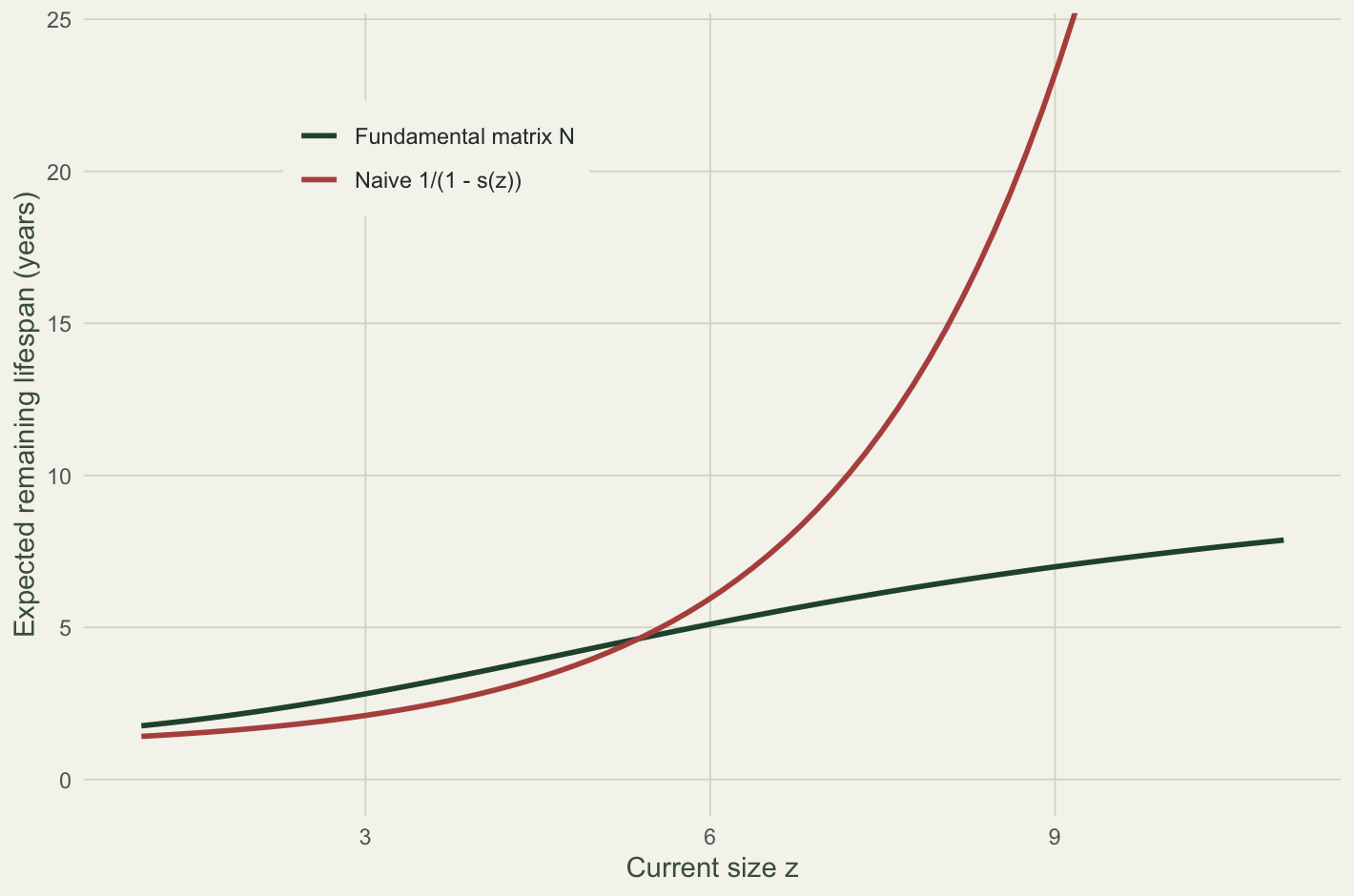
A recruit at size 2.2 has an expected 2.3 years ahead of it, not the 1.7 the shortcut gives: it will grow into sizes with better survival, so the shortcut is 25 per cent too low. At the other end the shortcut fails far worse in the opposite direction. A large plant at size 9 has annual survival 0.96, so 1 / (1 - s) suggests 24 years, but its true life expectancy is only 7. It does not stay large: it regresses towards the equilibrium size, where survival is lower, and its remaining life is governed by that whole downward trajectory rather than by the survival it happens to have today. The fundamental matrix integrates over the trajectory; the shortcut cannot.
First-passage time: how long to reach a size
The same operator answers a timing question, this time using growth alone. Treat the eviction-corrected growth as a size-to-size Markov chain among survivors, make every size at or above a target absorbing, and the fundamental matrix of the remaining transient block gives the expected number of years to first reach the target.
TG    <- G * h                                   # column-stochastic growth transition
zstar <- 5.5
absb  <- mesh >= zstar
Q     <- TG[!absb, !absb]
Ng    <- solve(diag(sum(!absb)) - Q)
pass  <- rep(0, m); pass[!absb] <- colSums(Ng)   # years to grow up to zstar

sapply(c(2.2, 3, 4, 5), function(z) round(pass[which.min(abs(mesh - z))], 2))
[1] 6.36 5.75 4.80 3.58d2 <- data.frame(z = mesh[!absb], years = pass[!absb])
ggplot(d2, aes(z, years)) +
geom_line(colour = te$forest, linewidth = 1) +
labs(x = "Starting size z", y = "Expected years to reach size 5.5") +
theme_te(11)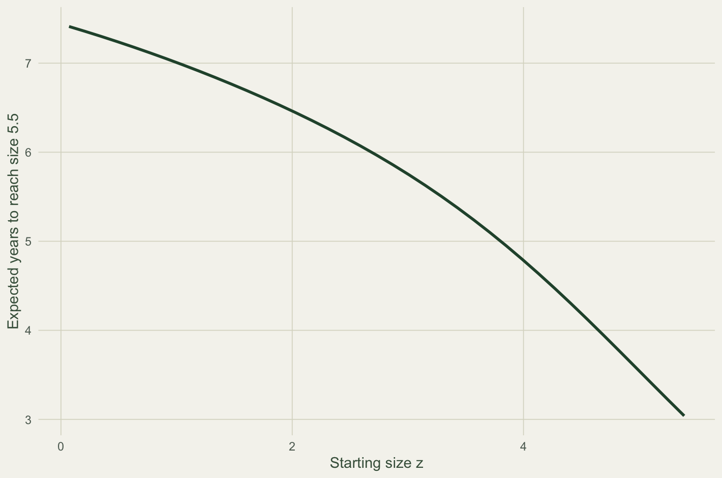
A surviving recruit takes about 6.4 years to reach size 5.5, falling to 3.6 years for a plant that starts at size 5. The curve does not drop to zero at the target because the growth equilibrium sits just below it: plants pile up a little under 5.5 and cross only on a lucky upward step, so even a large juvenile waits a few years. Targets above the equilibrium size are reached slowly and unreliably, which is itself a demographic fact worth knowing when the target is first reproduction.
From residence time to the fundamental matrix
The shortcut 1 / (1 - s) is not wrong so much as incomplete: it is the mean residence time of a single absorbing stage, the same quantity a Lefkovitch matrix reports as 1 / (1 - stasis). It works when an individual really does stay put. The moment size changes, life expectancy and passage time depend on the entire sequence of sizes an individual moves through, and that sequence is exactly what N = (I - P) inverse sums over. One solve() on the survival-growth block gives both, and both connect the IPM back to the survival and time-to-event questions of ordinary demography.
References
Cochran ME, Ellner S 1992. Ecological Monographs 62(3):345-364 (10.2307/2937115).
Caswell H 2001. Matrix Population Models. 2nd ed. Sinauer Associates. ISBN 978-0-87893-096-8.
Ellner SP, Rees M 2006. American Naturalist 167(3):410-428 (10.1086/499438).
Merow C, Dahlgren JP, Metcalf CJE, Childs DZ, Evans MEK, Jongejans E, Record S, Rees M, Salguero-Gomez R, McMahon SM 2014. Methods in Ecology and Evolution 5(2):99-110 (10.1111/2041-210X.12146).
Ellner SP, Childs DZ, Rees M 2016. Data-driven Modelling of Structured Populations. Springer. ISBN 978-3-319-28891-8.