Geographical detector: the interaction rule

The geographical detector calls independent, additive drivers a nonlinear enhancement in over half of datasets. Why, what q is, and where shift tests fail.

A land-cover study has an NDVI value for every cell of a raster and two candidate drivers for it, elevation and distance to the nearest road, each cut into five classes. A common next step in land-use and remote-sensing ecology is the geographical detector. Its factor detector gives each driver a q value, the share of the variance in NDVI that its classes explain. Its interaction detector then overlays the two classifications, computes q for the combined classes, and names the pair with one of five words. A verdict often seen in published tables is “nonlinear enhancement”: the two drivers together explain more than the sum of what they explain apart, and the discussion section reads that as a synergy between elevation and roads.

The q value itself is not the problem. It is the ratio of the between-class sum of squares to the total sum of squares, which is eta squared from a one-way analysis of variance, and it answers a sensible question about stratified heterogeneity (Wang et al. 2010; Wang, Zhang and Fu 2016). The problem is the rule that turns three q values into a verdict. This post measures how often that rule says “nonlinear enhancement” when the two drivers act on the response purely additively, with no interaction of any kind, and what decides the answer when it does.

The nearest posts on this site come at it from other sides. Variation partitioning in R warns that “Raw R-squared always rises as you add predictors, so a set with more columns looks more important purely from its size”, and splits two sets of predictors into unique and shared fractions; the shared fraction reappears below as half of the interaction rule. Interaction terms in ecological GLMs reads an interaction as a difference in slopes and shows that curves fanning apart on the count scale are not evidence of one; here there are no slopes, only class means. Natural breaks in QGIS and R is about how a continuous layer gets cut into classes in the first place, which is the step the detector takes for granted. The spatial half of the post leans on Spatial autocorrelation and Moran’s I in R for the diagnostic and on Two-species point patterns for the toroidal shift, which that post uses on point patterns and which is tried here on rasters. Permutation nulls that keep the map measures map-keeping nulls for the correlation between two maps on irregular sites; the question here is an interaction between two drivers on a regular grid, and the null is the shift rather than a spectral randomisation.

library(ggplot2)
library(splines)

te_paper  <- "#f5f4ee"
te_ink    <- "#16241d"
te_body   <- "#2c3a31"
te_forest <- "#275139"
te_rust   <- "#b5534e"
te_gold   <- "#c9b458"
te_line   <- "#dad9ca"

theme_datasheet <- function() {
  theme_minimal(base_size = 12) +
    theme(plot.background  = element_rect(fill = te_paper, colour = NA),
          panel.background = element_rect(fill = te_paper, colour = NA),
          panel.grid.major = element_line(colour = te_line, linewidth = 0.3),
          panel.grid.minor = element_blank(),
          text             = element_text(colour = te_body),
          plot.title       = element_text(colour = te_ink, face = "bold"),
          plot.subtitle    = element_text(colour = te_body),
          axis.text        = element_text(colour = te_body),
          strip.text       = element_text(colour = te_ink))
}

q is eta squared of a classification

Wang, Zhang and Fu (2016) write the statistic for a response of N units split into L classes as q = 1 - sum_h N_h sigma_h^2 / (N sigma^2), where N_h and sigma_h^2 are the size and variance of class h and sigma^2 is the variance of the whole response. With both variances taken with their own counts as divisors, N_h sigma_h^2 is the within-class sum of squares of class h, so q is one minus the within-class sum of squares over the total: the R-squared of a linear model with the class as a factor. The function below computes it from class sums, and the chunk checks it against lm().

disc_q <- function(x, n_class) {
  brk <- quantile(x, seq(0, 1, length.out = n_class + 1))
  as.integer(cut(x, brk, include.lowest = TRUE))
}
ss_within <- function(y, g) {
  n_g <- tabulate(g)
  n_g <- n_g[n_g > 0]
  sum(y^2) - sum(rowsum(y, g, reorder = TRUE)^2 / n_g)
}
q_stat <- function(y, g) 1 - ss_within(y, g) / sum((y - mean(y))^2)

n_class <- 5
set.seed(4301)
x_demo <- rnorm(200)
y_demo <- 0.5 * x_demo + rnorm(200)
g_demo <- disc_q(x_demo, n_class)
q_demo <- q_stat(y_demo, g_demo)
stopifnot(abs(q_demo - summary(lm(y_demo ~ factor(g_demo)))$r.squared) < 1e-12)

n_unit <- 1024
n_null <- 2000
null_q <- replicate(n_null, {
  y_n <- rnorm(n_unit)
  g1 <- disc_q(rnorm(n_unit), n_class)
  g2 <- disc_q(rnorm(n_unit), n_class)
  c(q1 = q_stat(y_n, g1), q12 = q_stat(y_n, (g1 - 1L) * n_class + g2),
    cells = length(unique((g1 - 1L) * n_class + g2)))
})
eq_one  <- (n_class - 1) / (n_unit - 1)
eq_two  <- (n_class^2 - 1) / (n_unit - 1)
null_m  <- rowMeans(null_q)
null_se <- apply(null_q, 1, sd) / sqrt(n_null)
stopifnot(all(null_q["cells", ] == n_class^2))

A classification explains some variance even when it is unrelated to the response, and how much has a closed form. With L classes and N units, the expected q of a classification drawn independently of the response is (L - 1) / (N - 1): under normal errors q follows a beta distribution with parameters (L - 1) / 2 and (N - L) / 2, and the same mean holds for any response under random reallocation of units to classes. For five classes and 1024 units that is 0.00391, and over 2000 simulated datasets with an unrelated response the mean q is 0.00396 (Monte Carlo standard error 0.00006). Overlaying two such classifications gives 25 combined classes, and the expected q rises to 24 / (N - 1) = 0.02346; the simulated mean is 0.02357 (standard error 0.00015). This is the size effect the varpart post warns about: more classes, more variance explained, with nothing behind it. Here the combined classification has six times the expected q of either of its parts before any driver has done anything.

The rule and the identity it compares against

The interaction detector of Wang et al. (2010) computes q1 and q2 for the two classifications and q12 for the classification formed by every combination of their classes, and compares q12 with q1, q2 and q1 + q2. That paper lists seven relations, and they overlap: a q12 above the larger q but below the sum is there both an “enhance, bi-” (larger than each driver alone) and a “weaken” (smaller than the sum). Current software reduces them to five mutually exclusive types. The coding below follows the order of tests in gdinteract() of the GD package, version 10.9 (Song et al. 2020), whose source was read for this post: q12 below the smaller of q1 and q2 is a nonlinear weakening; between the two is a univariate weakening; above the larger but below q1 + q2 is a bivariate enhancement; exactly q1 + q2 is independence; above q1 + q2 is a nonlinear enhancement.

gd_verdict <- function(q1, q2, q12) {
  ifelse(q12 < pmin(q1, q2), "weaken, nonlinear",
  ifelse(q12 <= pmax(q1, q2), "weaken, uni-",
  ifelse(q12 < q1 + q2, "enhance, bi-",
  ifelse(q12 == q1 + q2, "independent", "enhance, nonlinear"))))
}
verdict_levels <- c("enhance, nonlinear", "independent", "enhance, bi-",
                    "weaken, uni-", "weaken, nonlinear")

# population q of one quintile classification of a standard normal driver
cut_pts <- qnorm(seq(0, 1, length.out = n_class + 1))
cls_mean <- (dnorm(cut_pts[-(n_class + 1)]) - dnorm(cut_pts[-1])) * n_class
v_between <- mean(cls_mean^2)
b_set <- c(0, 0.25, 0.5, 1)
q_pop <- b_set^2 * v_between / (2 * b_set^2 + 1)

gd_pieces <- function(y, g1, g2) {
  g12 <- (g1 - 1L) * n_class + g2
  sst <- sum((y - mean(y))^2)
  sse_cell <- ss_within(y, g12)
  x_add <- cbind(1, outer(g1, 2:n_class, "==") + 0, outer(g2, 2:n_class, "==") + 0)
  sse_add <- sum(.lm.fit(x_add, y)$residuals^2)
  n_cell <- length(unique(g12))
  df_ab <- n_cell - 2 * n_class + 1
  df_e  <- length(y) - n_cell
  f_ab  <- ((sse_add - sse_cell) / df_ab) / (sse_cell / df_e)
  n_g <- tabulate(g12)
  c(q1 = q_stat(y, g1), q2 = q_stat(y, g2), q12 = 1 - sse_cell / sst,
    q_add = 1 - sse_add / sst, f_p = pf(f_ab, df_ab, df_e, lower.tail = FALSE),
    single = sum(n_g == 1))
}

set.seed(4302)
n_big <- 2^20
x1_big <- rnorm(n_big)
x2_big <- rnorm(n_big)
y_big  <- 0.5 * x1_big + 0.5 * x2_big + rnorm(n_big)
big <- gd_pieces(y_big, disc_q(x1_big, n_class), disc_q(x2_big, n_class))
big_gap <- big[["q12"]] - big[["q1"]] - big[["q2"]]
stopifnot(abs((big[["q12"]] - big[["q1"]] - big[["q2"]]) -
              ((big[["q12"]] - big[["q_add"]]) - (big[["q1"]] + big[["q2"]] - big[["q_add"]]))) < 1e-12)

For two drivers that act additively and independently, the population value of q12 is exactly q1 + q2. Write the response as y = f1(x1) + f2(x2) + e. The between-class variance of the combined classes is the variance of E[y | class of x1, class of x2], which is E[f1 | class of x1] + E[f2 | class of x2] plus a constant, because the class of x2 carries no information about x1. The two terms are independent, so their variances add, and dividing by the variance of y gives q12 = q1 + q2. This is an identity of the population, not a simulation result, and the “independent” verdict is the one the rule reserves for it. An estimate never lands on an equality between continuous quantities, so for additive independent drivers the rule has to pick one of the other four words.

In fact it has only two to choose from. Every combined class lies inside one class of x1 and one class of x2, so splitting the units into combined classes can only lower the within-class sum of squares of either single classification, never raise it. On the same units q12 is therefore at least as large as the larger of q1 and q2, and the two weakening types cannot occur. The GD code drops classes that hold a single unit before computing each q, which changes the units behind q12 and is one route by which a weakening could appear there; missing driver values are another, because GD drops those units from the within-class sum of a single driver but keeps them in its total, and keeps them as classes of their own in the combined one. Here q is computed on all units, as the formula defines it, and every simulated dataset below is checked for the inequality.

With y = 0.5 x1 + 0.5 x2 + e and quintile classes of standard normal drivers, the population q of each driver is 0.1495, from the class means of a normal in closed form. One dataset of 1048576 units gives q1 = 0.1505, q2 = 0.1503 and q12 = 0.3005, and q12 - q1 - q2 = -0.00033.

What decides the sign of q12 - q1 - q2 in a finite sample is an exact split into two pieces. Let q_add be the R-squared of the additive two-way model with both classifications as factors and no interaction. Then q12 - q1 - q2 = (q12 - q_add) - (q1 + q2 - q_add). The first piece is the interaction sum of squares of a two-way analysis of variance on the same classes, divided by the total; it can never be negative, because the additive model is nested in the combined-class model. The second piece is the raw shared fraction of variation partitioning, the part of the explained variance that the two classifications claim twice. The rule says “nonlinear enhancement” exactly when the interaction piece beats the shared piece. The stopifnot() in the chunk checks the split on the large dataset.

Additive drivers, read as enhancing

The design below is fixed before running: two independent standard normal drivers, quintile classes, y = b x1 + b x2 + e with standard normal e, and b of 0, 0.25, 0.5 and 1, so that each driver’s population q runs from zero to 0.299. Every dataset is run through the rule and through the interaction F test of the two-way analysis of variance on the same classes, which is the standard test of the question the rule is trying to answer.

n_set <- c(256, 1024, 4096, 16384)
n_rep <- 400
set.seed(4303)
rate_raw <- do.call(rbind, lapply(n_set, function(nn) do.call(rbind, lapply(b_set, function(bb) {
  out <- t(replicate(n_rep, {
    x1 <- rnorm(nn)
    x2 <- rnorm(nn)
    gd_pieces(bb * x1 + bb * x2 + rnorm(nn), disc_q(x1, n_class), disc_q(x2, n_class))
  }))
  data.frame(n = nn, b = bb, out)
}))))
stopifnot(all(rate_raw$q12 >= pmax(rate_raw$q1, rate_raw$q2) - 1e-12))
rate_raw$verdict <- gd_verdict(rate_raw$q1, rate_raw$q2, rate_raw$q12)
rate_raw$enh <- rate_raw$verdict == "enhance, nonlinear"
rate_raw$f_rej <- rate_raw$f_p < 0.05
rate_tab <- aggregate(cbind(enh, f_rej, q1) ~ n + b, rate_raw, mean)
rt <- function(nn, bb, v) rate_tab[rate_tab$n == nn & rate_tab$b == bb, v]
mc_se_max <- sqrt(0.25 / n_rep)
n_indep <- sum(rate_raw$verdict == "independent")
f_range <- range(rate_tab$f_rej)
f_se <- sqrt(0.05 * 0.95 / n_rep)

Each rate below comes from 400 datasets, so its Monte Carlo standard error is at most 0.025. At 1024 units and b = 0.5, where each driver explains about 15 per cent of the variance, the rule reports a nonlinear enhancement in 86.0 per cent of datasets. With no effect at all, b = 0, it does so in 100.0 per cent, and at b = 0.25 in 99.2 per cent. The verdict “independent” came up 0 times in 6400 datasets.

More data does not rescue the rule. At 16384 units the rate is 59.2 per cent for b = 0.5 and 52.0 per cent for b = 1, while for b = 0 it is still 100.0 per cent. The interaction F test on the same datasets rejects at the five per cent level in 3.3 to 5.7 per cent of the datasets across all sixteen combinations of N and b; a single rate of five per cent would have a Monte Carlo standard error of 0.011.

rate_long <- rbind(
  data.frame(rate_tab[, c("n", "b")], panel = "rule: nonlinear enhancement", rate = rate_tab$enh),
  data.frame(rate_tab[, c("n", "b")], panel = "interaction F test, p < 0.05", rate = rate_tab$f_rej))
rate_long$panel <- factor(rate_long$panel, c("rule: nonlinear enhancement", "interaction F test, p < 0.05"))
rate_long$b_lab <- factor(sprintf("b = %.2f, q = %.3f", rate_long$b, q_pop[match(rate_long$b, b_set)]))
ref_df <- data.frame(panel = factor(levels(rate_long$panel), levels(rate_long$panel)), y_ref = c(0.5, 0.05))
lim_df <- data.frame(panel = factor(rep(levels(rate_long$panel), each = 2), levels(rate_long$panel)),
                     n = n_set[1], rate = c(0.4, 1, 0, 0.1))

ggplot(rate_long, aes(n, rate, colour = b_lab)) +
  geom_hline(data = ref_df, aes(yintercept = y_ref), linetype = "dashed",
             colour = te_body, linewidth = 0.5) +
  geom_blank(data = lim_df, aes(n, rate), inherit.aes = FALSE) +
  geom_line(linewidth = 0.9) +
  geom_point(size = 2.2) +
  facet_wrap(~ panel, scales = "free_y") +
  scale_x_log10(breaks = n_set) +
  scale_colour_manual(values = c(te_ink, te_forest, te_gold, te_rust), name = NULL) +
  labs(x = "units (log scale)", y = "share of datasets",
       title = "Additive drivers, read as a synergy") +
  theme_datasheet() +
  theme(legend.position = "bottom") +
  guides(colour = guide_legend(nrow = 2))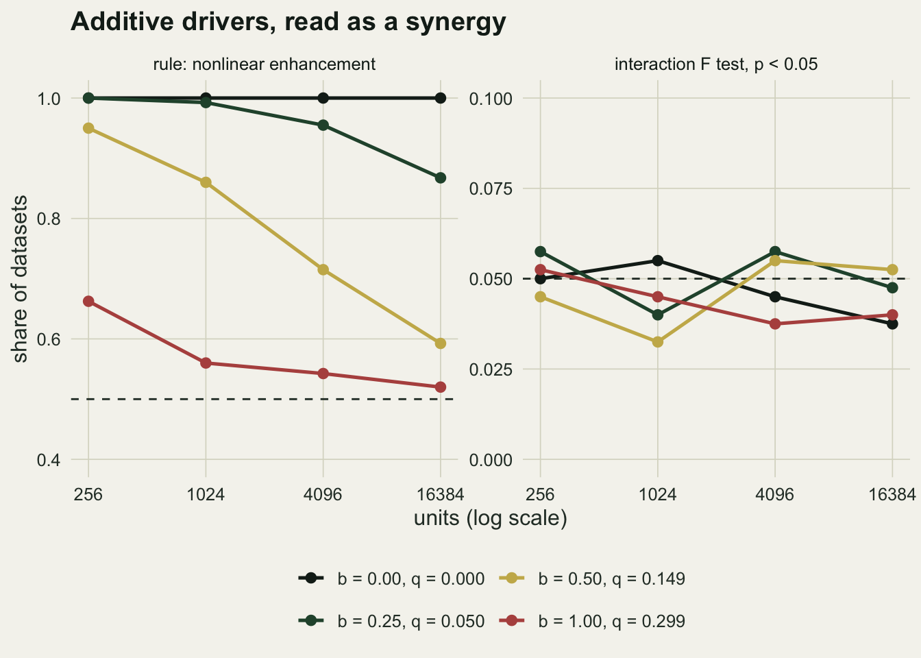

Figure 1: Share of datasets with two independent, additive drivers that the interaction rule calls a nonlinear enhancement (left) and that the two-way interaction F test rejects at the five per cent level (right), by number of units and effect size b. Each point is 400 datasets.

The split into an interaction piece and a shared piece says why. The interaction piece is never negative and, with no interaction, it is the share of the variance picked up by the (L - 1)^2 = 16 interaction degrees of freedom out of the variance the additive model leaves unexplained, so its expected size is about 16 / (N - 1) times one minus q_add. The shared piece would be exactly zero if the counts in the 25 combined classes were exactly proportional to the class totals, because the two classifications would then be orthogonal factors and their sums of squares would add. With independent drivers the counts are proportional only in expectation, and in any one dataset they wander from it; that makes the shared piece positive in some datasets and negative in others, by an amount that grows with the size of the effects.

dec <- rate_raw[rate_raw$b == 0.5 & rate_raw$n %in% c(1024, 16384), ]
dec$inter  <- dec$q12 - dec$q_add
dec$shared <- dec$q1 + dec$q2 - dec$q_add
stopifnot(all(dec$inter >= 0), all(dec$enh == (dec$inter > dec$shared)))
dec_tab <- aggregate(cbind(inter, shared, q_add) ~ n, dec, mean)
dec_sd  <- aggregate(shared ~ n, dec, sd)
dec_pos <- aggregate(shared ~ n, dec, function(v) mean(v > 0))
dk <- function(nn, tb, v) tb[tb$n == nn, v]
ratio_1k  <- dk(1024, dec_tab, "inter") / dk(1024, dec_sd, "shared")
ratio_16k <- dk(16384, dec_tab, "inter") / dk(16384, dec_sd, "shared")
inter_expect <- (n_class - 1)^2 / (1024 - 1) * (1 - dk(1024, dec_tab, "q_add"))
shared_se_1k <- dk(1024, dec_sd, "shared") / sqrt(n_rep)

sub_1k <- rate_raw[rate_raw$n == 1024, ]
sub_1k$inter  <- sub_1k$q12 - sub_1k$q_add
sub_1k$shared <- sub_1k$q1 + sub_1k$q2 - sub_1k$q_add
by_b <- data.frame(b = b_set,
  inter = tapply(sub_1k$inter, sub_1k$b, mean),
  shared_sd = tapply(sub_1k$shared, sub_1k$b, sd))

g_bal1 <- rep(1:n_class, each = 200)
g_bal2 <- rep(rep(1:n_class, each = 40), n_class)
stopifnot(all(table(g_bal1, g_bal2) == 40))
set.seed(4309)
y_bal <- 0.5 * g_bal1 + 0.5 * g_bal2 + rnorm(length(g_bal1))
bal <- gd_pieces(y_bal, g_bal1, g_bal2)
bal_shared <- bal[["q1"]] + bal[["q2"]] - bal[["q_add"]]
stopifnot(abs(bal_shared) < 1e-12)

On a balanced design with exactly 40 units in every combined class the shared piece is zero to rounding error; the stopifnot() in the chunk requires it to be below one part in a trillion. On the simulated datasets at 1024 units its standard deviation is 0.00021 with no effect, 0.0034 at b = 0.25, 0.0090 at b = 0.5 and 0.0198 at b = 1, while the mean interaction piece is 0.0155, 0.0137, 0.0109 and 0.0062. With no effect the shared piece is far smaller than the interaction piece and the rule says “nonlinear enhancement” every time; as the effect grows the shared piece catches up, and at b = 1 its standard deviation is the larger of the two.

At b = 0.5 the mean interaction piece is 0.0109 at 1024 units, against 0.0109 from 16 / (N - 1) times one minus the mean q_add, and 0.00067 at 16384, falling roughly as 1 / N. The shared piece has a mean of -0.00008 (Monte Carlo standard error 0.00045) and a standard deviation of 0.0090 at 1024 units, and +0.00004 and 0.00240 at 16384; it is positive in 48.2 and 51.5 per cent of datasets. The ratio of the mean interaction piece to that standard deviation drops from 1.21 to 0.28: the interaction piece shrinks like 1 / N and the shared piece like one over the square root of N, so with enough units the verdict turns on the sign of the shared piece, and that sign is set by chance. The rate of “nonlinear enhancement” heads for one half, not for zero.

dec$n_lab <- factor(sprintf("%d units", dec$n), sprintf("%d units", c(1024, 16384)))
dec$verdict <- factor(dec$verdict, verdict_levels)
ggplot(dec, aes(shared, inter, colour = verdict)) +
  geom_abline(slope = 1, intercept = 0, colour = te_body, linewidth = 0.5) +
  geom_vline(xintercept = 0, colour = te_line, linewidth = 0.6) +
  geom_point(size = 1.4, alpha = 0.7) +
  facet_wrap(~ n_lab, scales = "free") +
  scale_colour_manual(values = c("enhance, nonlinear" = te_rust, "enhance, bi-" = te_gold),
                      drop = TRUE, name = NULL) +
  labs(x = "shared piece, q1 + q2 - q_add", y = "interaction piece, q12 - q_add",
       title = "A positive term against a coin flip") +
  theme_datasheet() +
  theme(legend.position = "bottom", plot.margin = margin(5.5, 18, 5.5, 5.5))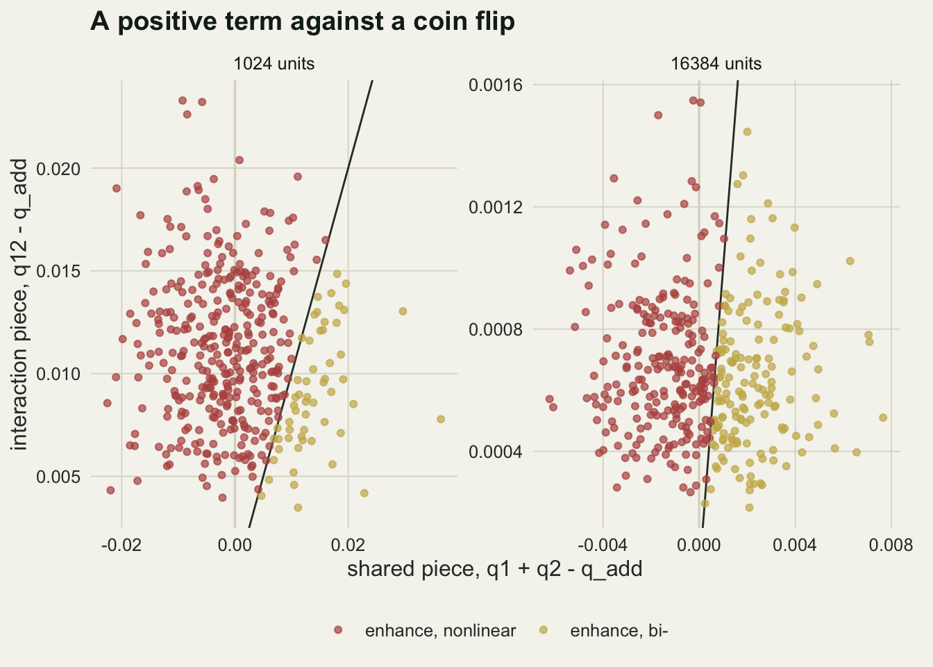

Figure 2: The interaction piece against the shared piece for each dataset at b = 0.5. Points above the diagonal are called a nonlinear enhancement, points below it a bivariate enhancement. The panels have different scales.

Correlated drivers: the sign decides

Real drivers are rarely independent. Roads follow valleys, so elevation and distance to roads tend to be correlated, and temperature and elevation strongly so. Correlation between the drivers feeds the shared piece directly. When the two contributions to the response are positively correlated, the two classifications explain overlapping variance, so q1 + q2 exceeds q_add and the shared piece moves above zero. When the contributions are negatively correlated, each classification hides part of what the other explains, and the shared piece goes below zero. The run below keeps the additive model, b = 0.5 and 1024 units, and correlates the two normal drivers at r from 0 to 0.5, and at r = -0.5. With both effects positive, r = -0.5 is the case of elevation raising NDVI while distance to roads, positively correlated with elevation, lowers it: reversing the sign of one driver only reverses the order of its classes, which changes no q, and the chunk checks this on one dataset.

rho_set <- c(0, 0.1, 0.2, 0.3, 0.5, -0.5)
set.seed(4304)
cor_raw <- do.call(rbind, lapply(rho_set, function(rho) {
  out <- t(replicate(n_rep, {
    x1 <- rnorm(n_unit)
    x2 <- rho * x1 + sqrt(1 - rho^2) * rnorm(n_unit)
    gd_pieces(0.5 * x1 + 0.5 * x2 + rnorm(n_unit), disc_q(x1, n_class), disc_q(x2, n_class))
  }))
  data.frame(rho = rho, out)
}))
cor_raw$verdict <- gd_verdict(cor_raw$q1, cor_raw$q2, cor_raw$q12)
cor_raw$enh <- cor_raw$verdict == "enhance, nonlinear"
cor_raw$bi  <- cor_raw$verdict == "enhance, bi-"
cor_raw$shared <- cor_raw$q1 + cor_raw$q2 - cor_raw$q_add
cor_raw$f_rej <- cor_raw$f_p < 0.05
cor_raw$shared_pos <- cor_raw$shared > 0
cor_tab <- aggregate(cbind(enh, bi, shared, shared_pos, f_rej) ~ rho, cor_raw, mean)
stopifnot(all(cor_raw$bi[cor_raw$rho >= 0.2]), all(cor_raw$shared_pos[cor_raw$rho >= 0.2]))
ct <- function(rr, v) cor_tab[cor_tab$rho == rr, v]
stopifnot(all(cor_raw$enh[cor_raw$rho == -0.5]), all(cor_raw$shared[cor_raw$rho == -0.5] < 0))

set.seed(4313)
x1_flip <- rnorm(n_unit)
x2_flip <- -0.5 * x1_flip + sqrt(0.75) * rnorm(n_unit)
y_flip  <- 0.5 * x1_flip + 0.5 * x2_flip + rnorm(n_unit)
flip_a <- gd_pieces(y_flip, disc_q(x1_flip, n_class), disc_q(x2_flip, n_class))
flip_b <- gd_pieces(y_flip, disc_q(x1_flip, n_class), disc_q(-x2_flip, n_class))
stopifnot(max(abs(flip_a[1:4] - flip_b[1:4])) < 1e-12)

spline_f <- function(y, x1, x2) {
  b1 <- ns(x1, df = 4)
  b2 <- ns(x2, df = 4)
  x_a <- cbind(1, b1, b2)
  x_i <- cbind(x_a, do.call(cbind, lapply(1:4, function(j) b1[, j] * b2)))
  rss_a <- sum(.lm.fit(x_a, y)$residuals^2)
  rss_i <- sum(.lm.fit(x_i, y)$residuals^2)
  df_i <- ncol(x_i) - ncol(x_a)
  pf(((rss_a - rss_i) / df_i) / (rss_i / (length(y) - ncol(x_i))), df_i,
     length(y) - ncol(x_i), lower.tail = FALSE)
}
set.seed(4305)
cls_vs_spline <- do.call(rbind, lapply(c(1024, 4096), function(nn) {
  out <- t(replicate(n_rep, {
    x1 <- rnorm(nn)
    x2 <- 0.5 * x1 + sqrt(0.75) * rnorm(nn)
    y <- 0.5 * x1 + 0.5 * x2 + rnorm(nn)
    c(cls = gd_pieces(y, disc_q(x1, n_class), disc_q(x2, n_class))[["f_p"]] < 0.05,
      spl = spline_f(y, x1, x2) < 0.05)
  }))
  data.frame(n = nn, cls = mean(out[, "cls"]), spl = mean(out[, "spl"]))
}))

set.seed(4312)
cls_big <- do.call(rbind, lapply(c(0.1, 0.2), function(rho) {
  rej <- replicate(n_rep, {
    x1 <- rnorm(16384)
    x2 <- rho * x1 + sqrt(1 - rho^2) * rnorm(16384)
    gd_pieces(0.5 * x1 + 0.5 * x2 + rnorm(16384), disc_q(x1, n_class), disc_q(x2, n_class))[["f_p"]] < 0.05
  })
  data.frame(rho = rho, f_rej = mean(rej))
}))

At r = 0.1 the rule already calls 5.7 per cent of datasets a nonlinear enhancement and 94.3 per cent a bivariate one, against 82.8 and 17.2 per cent at r = 0 on this run’s own draws; the mean shared piece has grown from +0.0012 to 0.0290. The shared piece is positive in 52.5 per cent of datasets at r = 0 and in 100.0 per cent at r = 0.1. From r = 0.2 upwards every dataset is a bivariate enhancement, and at r = 0.5 the shared piece averages 0.182. At r = -0.5 it averages -0.074 and is negative in every dataset, and the rule calls 100.0 per cent of them a nonlinear enhancement. Same process, same absence of interaction: the verdict follows the sign of the correlation between the two contributions, not any interaction.

The interaction F test on classes has a problem of its own here. When the drivers are correlated, the mean of x1 inside a class of x1 depends on which class of x2 the unit is in, so the class means of an additive response are no longer additive in the two classifications. The classes carry a real interaction that the process does not have. It is a property of the class means, not of the sample, so the F test finds it more often as N grows: with r = 0.5, in the draws used for the spline comparison below, it rejects in 9.0 per cent of datasets at 1024 units and 31.0 per cent at 4096. At 1024 units and r from 0 to 0.5 its rejection rates in the main run are 5.2, 5.2, 5.7, 6.2 and 8.3 per cent. At 16384 units a correlation of 0.1 gives 6.0 per cent and a correlation of 0.2 gives 12.8 per cent, each from 400 datasets. A test on the continuous drivers does not have this problem. Comparing an additive model with a natural spline of four degrees of freedom in each driver against the same model plus their tensor-product terms, the interaction F test rejects in 3.5 and 4.0 per cent of the same kind of datasets. Once the drivers are correlated, cutting them into classes costs the interaction question its meaning, and the model should use the drivers as measured.

On a raster, the units are not independent

Everything so far treated the units as independent draws. A raster is not that: neighbouring cells share their elevation, their NDVI and their distance to a road. The grids below are 32 by 32 cells, 1024 units as before, and each layer (the two drivers and the error) is Gaussian noise smoothed with a Gaussian kernel whose standard deviation is r cells, then standardised. The fields are generated on a larger wrapped grid and a 32 by 32 window is cut out, so the window does not wrap at its edges, as a real map does not. Two ranges are used: a kernel standard deviation of 2 cells and of 5 cells.

n_side <- 32
r_set  <- c(2, 5)
smooth_layer <- function(n, r, wrap = FALSE) {
  m <- if (wrap) n else n + ceiling(4 * r)
  w <- matrix(rnorm(m * m), m, m)
  d_wrap <- pmin(0:(m - 1), m - 0:(m - 1))
  k_one <- exp(-d_wrap^2 / (2 * r^2))
  z <- Re(fft(fft(w) * fft(outer(k_one, k_one)), inverse = TRUE))[1:n, 1:n]
  as.vector((z - mean(z)) / sd(as.vector(z)))
}
moran_rook <- function(v, n) {
  z <- matrix(v - mean(v), n, n)
  cross <- sum(z[-1, ] * z[-n, ]) + sum(z[, -1] * z[, -n])
  (n * n / (4 * n * (n - 1))) * 2 * cross / sum(z^2)
}
set.seed(4306)
map_df <- do.call(rbind, lapply(r_set, function(r) {
  x1 <- smooth_layer(n_side, r)
  x2 <- smooth_layer(n_side, r)
  e  <- smooth_layer(n_side, r)
  y  <- 0.5 * x1 + 0.5 * x2 + e
  data.frame(r = r, row_i = rep(seq_len(n_side), n_side), col_i = rep(seq_len(n_side), each = n_side),
             layer = rep(c("driver x1", "driver x2", "response y"), each = n_side^2),
             value = c(x1, x2, as.vector(scale(y))))
}))

map_df$r_lab <- factor(sprintf("kernel SD %d cells", map_df$r), sprintf("kernel SD %d cells", r_set))
ggplot(map_df, aes(col_i, row_i, fill = value)) +
  geom_raster() +
  facet_grid(r_lab ~ layer) +
  scale_fill_gradient2(low = te_forest, mid = te_paper, high = te_rust, midpoint = 0,
                       name = "standardised value") +
  coord_equal(expand = FALSE) +
  labs(x = NULL, y = NULL, title = "Two ranges of spatial structure") +
  theme_datasheet() +
  theme(axis.text = element_blank(), panel.grid.major = element_blank(),
        legend.position = "bottom")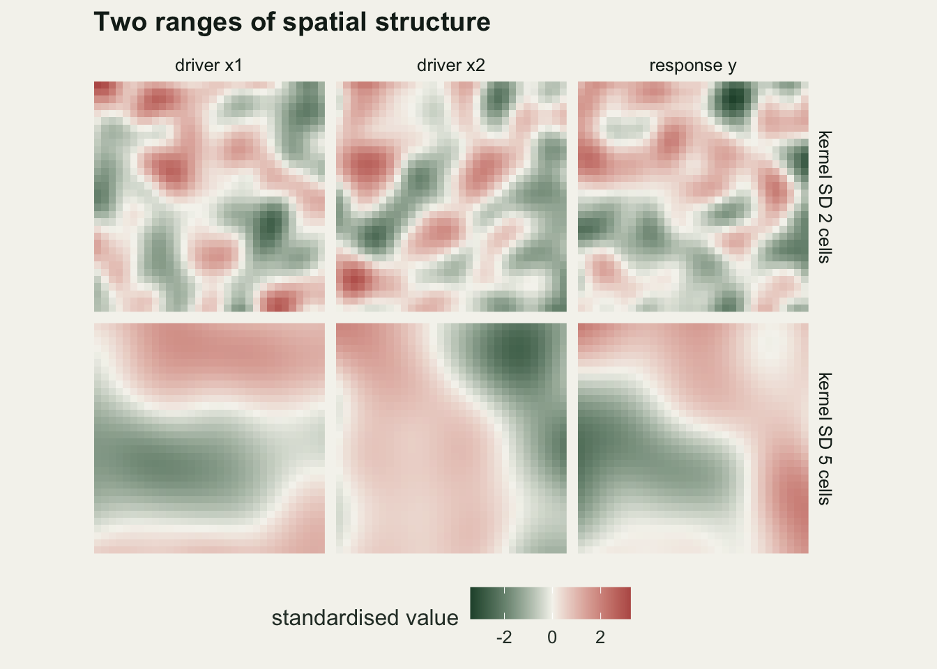

Figure 3: One simulated raster at each range: two independent drivers and an additive response, each standardised. Top row kernel standard deviation 2 cells, bottom row 5 cells.

Three scenarios run on these grids. In the null scenario the response is the error layer alone and has nothing to do with either driver. In the additive scenario it is 0.5 x1 + 0.5 x2 + e, as before. In the product scenario a real interaction, 0.5 x1 x2, is added, so that there is something for a test to find.

Two spatial versions of the interaction test are tried, both built on the toroidal shift that Lotwick and Silverman (1982) introduced for point patterns and that the point-pattern post uses. The observed statistic is the interaction F of the two-way analysis of variance on the classes; only its reference distribution changes. The driver shift slides the x2 layer, with its classes, over the grid by a random offset, wrapping at the edges, and recomputes F against the unmoved y and x1; this keeps each layer’s own spatial structure and breaks their alignment. The residual shift fits the additive two-way model, slides the map of its residuals instead, adds the shifted residuals back to the fitted values and recomputes F. Both use 99 shifts and reject when the observed F is among the five largest of the 100 values. Neither was run before this post was planned, and neither was adjusted after the results came in.

f_inter <- function(ymat, g1, g2) {
  g12 <- (g1 - 1L) * n_class + g2
  x_add <- cbind(1, outer(g1, 2:n_class, "==") + 0, outer(g2, 2:n_class, "==") + 0)
  sse_add <- colSums(qr.resid(qr(x_add), ymat)^2)
  n_g <- tabulate(g12)
  n_g <- n_g[n_g > 0]
  sse_cell <- colSums(ymat^2) - colSums(rowsum(ymat, g12, reorder = TRUE)^2 / n_g)
  df_ab <- length(n_g) - 2 * n_class + 1
  df_e  <- nrow(ymat) - length(n_g)
  ((sse_add - sse_cell) / df_ab) / (sse_cell / df_e)
}
shift_index <- function(n, dx, dy) {
  rr <- ((0:(n - 1) + dx) %% n) + 1
  cc <- ((0:(n - 1) + dy) %% n) + 1
  as.vector(outer(rr, (cc - 1) * n, "+"))
}
n_shift <- 99
one_grid <- function(scn, r, wrap = FALSE) {
  x1 <- smooth_layer(n_side, r, wrap)
  x2 <- smooth_layer(n_side, r, wrap)
  e  <- smooth_layer(n_side, r, wrap)
  y <- switch(scn, null = e, additive = 0.5 * x1 + 0.5 * x2 + e,
              product = 0.5 * x1 + 0.5 * x2 + 0.5 * x1 * x2 + e)
  g1 <- disc_q(x1, n_class)
  g2 <- disc_q(x2, n_class)
  pc <- gd_pieces(y, g1, g2)
  f_obs <- f_inter(matrix(y), g1, g2)
  s_id <- sample.int(n_side^2 - 1, n_shift)
  dx <- s_id %/% n_side
  dy <- s_id %% n_side
  f_drv <- vapply(seq_len(n_shift), function(i)
    f_inter(matrix(y), g1, g2[shift_index(n_side, dx[i], dy[i])]), 0)
  x_add <- cbind(1, outer(g1, 2:n_class, "==") + 0, outer(g2, 2:n_class, "==") + 0)
  fit_add <- qr.fitted(qr(x_add), y)
  res_add <- y - fit_add
  y_star <- vapply(seq_len(n_shift), function(i)
    fit_add + res_add[shift_index(n_side, dx[i], dy[i])], numeric(n_side^2))
  f_res <- f_inter(y_star, g1, g2)
  p_one <- pf((pc[["q1"]] / (n_class - 1)) / ((1 - pc[["q1"]]) / (n_side^2 - n_class)),
              n_class - 1, n_side^2 - n_class, lower.tail = FALSE)
  c(pc, moran = moran_rook(y, n_side), q1_rej = p_one < 0.05,
    drv_rej = sum(f_drv >= f_obs) + 1 <= 5, res_rej = sum(f_res >= f_obs) + 1 <= 5)
}
n_grid_rep <- 200
scn_set <- c("null", "additive", "product")
set.seed(4307)
grid_raw <- do.call(rbind, lapply(r_set, function(r) do.call(rbind, lapply(scn_set, function(scn)
  data.frame(r = r, scn = scn, t(replicate(n_grid_rep, one_grid(scn, r))))))))
grid_raw$verdict <- gd_verdict(grid_raw$q1, grid_raw$q2, grid_raw$q12)
grid_raw$enh <- grid_raw$verdict == "enhance, nonlinear"
grid_raw$f_rej <- grid_raw$f_p < 0.05
grid_tab <- aggregate(cbind(enh, f_rej, drv_rej, res_rej, q1_rej, q1, moran) ~ r + scn, grid_raw, mean)
gt <- function(r, scn, v) grid_tab[grid_tab$r == r & grid_tab$scn == scn, v]
grid_se <- sqrt(0.05 * 0.95 / n_grid_rep)
stopifnot(all(grid_raw$q12 >= pmax(grid_raw$q1, grid_raw$q2) - 1e-12))

set.seed(4310)
wrap_raw <- do.call(rbind, lapply(c("null", "additive"), function(scn)
  data.frame(scn = scn, t(replicate(n_grid_rep, one_grid(scn, 5, wrap = TRUE))))))
wrap_tab <- aggregate(cbind(drv_rej, res_rej, moran) ~ scn, wrap_raw, mean)
wt <- function(scn, v) wrap_tab[wrap_tab$scn == scn, v]
se_diff <- function(p1, p2) sqrt(p1 * (1 - p1) / n_grid_rep + p2 * (1 - p2) / n_grid_rep)
res_drop_z <- sapply(c("null", "additive"), function(scn)
  (gt(5, scn, "res_rej") - wt(scn, "res_rej")) / se_diff(gt(5, scn, "res_rej"), wt(scn, "res_rej")))
drv_drop_z <- sapply(c("null", "additive"), function(scn)
  (gt(5, scn, "drv_rej") - wt(scn, "drv_rej")) / se_diff(gt(5, scn, "drv_rej"), wt(scn, "drv_rej")))

Moran’s I of the response, with rook neighbours, averages 0.93 in the null scenario at a kernel standard deviation of 2 cells and 0.98 at 5 cells, against an expectation near zero for independent cells. The factor detector feels this first. In the null scenario the mean q of a driver that has nothing to do with the response is 0.0400 at the short range and 0.1310 at the long one, 10 and 34 times the independence value of 0.0039, and the one-way F test of that q rejects at the five per cent level in 86.5 and 98.5 per cent of grids. Two smooth maps that are unrelated still share large patches, and a classification of one explains the other’s patches.

The interaction rule does no better. In the null scenario it reports a nonlinear enhancement in 99.5 per cent of grids at the short range and 90.5 per cent at the long one; in the additive scenario in 76.0 and 65.0 per cent. The ordinary interaction F test, which held its level on independent units, now rejects in 89.5 and 100.0 per cent of null grids and 92.0 and 100.0 per cent of additive ones. It is the right question with the wrong reference distribution.

test_cols <- c(enh = "rule: nonlinear enhancement", f_rej = "interaction F test",
               drv_rej = "driver shift", res_rej = "residual shift")
sp_long <- do.call(rbind, lapply(names(test_cols), function(tc)
  data.frame(grid_tab[, c("r", "scn")], test = test_cols[[tc]], rate = grid_tab[[tc]])))
sp_long$se <- sqrt(sp_long$rate * (1 - sp_long$rate) / n_grid_rep)
sp_long$test <- factor(sp_long$test, rev(test_cols))
sp_long$scn  <- factor(sp_long$scn, scn_set, c("null: y unrelated", "additive", "product: real interaction"))
sp_long$r_lab <- factor(sprintf("kernel SD %d cells", sp_long$r), sprintf("kernel SD %d cells", r_set))

ggplot(sp_long, aes(rate, test, colour = r_lab)) +
  geom_vline(xintercept = 0.05, linetype = "dashed", colour = te_body, linewidth = 0.5) +
  geom_errorbar(aes(xmin = pmax(rate - 2 * se, 0), xmax = pmin(rate + 2 * se, 1)),
                orientation = "y", width = 0.25, linewidth = 0.6,
                position = position_dodge(width = 0.55)) +
  geom_point(size = 2.4, position = position_dodge(width = 0.55)) +
  facet_wrap(~ scn, ncol = 3) +
  scale_colour_manual(values = c(te_forest, te_rust), name = NULL) +
  scale_x_continuous(limits = c(0, 1), breaks = c(0, 0.5, 1), labels = c("0", "0.5", "1")) +
  labs(x = "share of rasters reporting an interaction", y = NULL,
       title = "Only the shift tests come near 5%, at short range") +
  theme_datasheet() +
  theme(legend.position = "bottom", panel.spacing.x = unit(1.2, "lines"))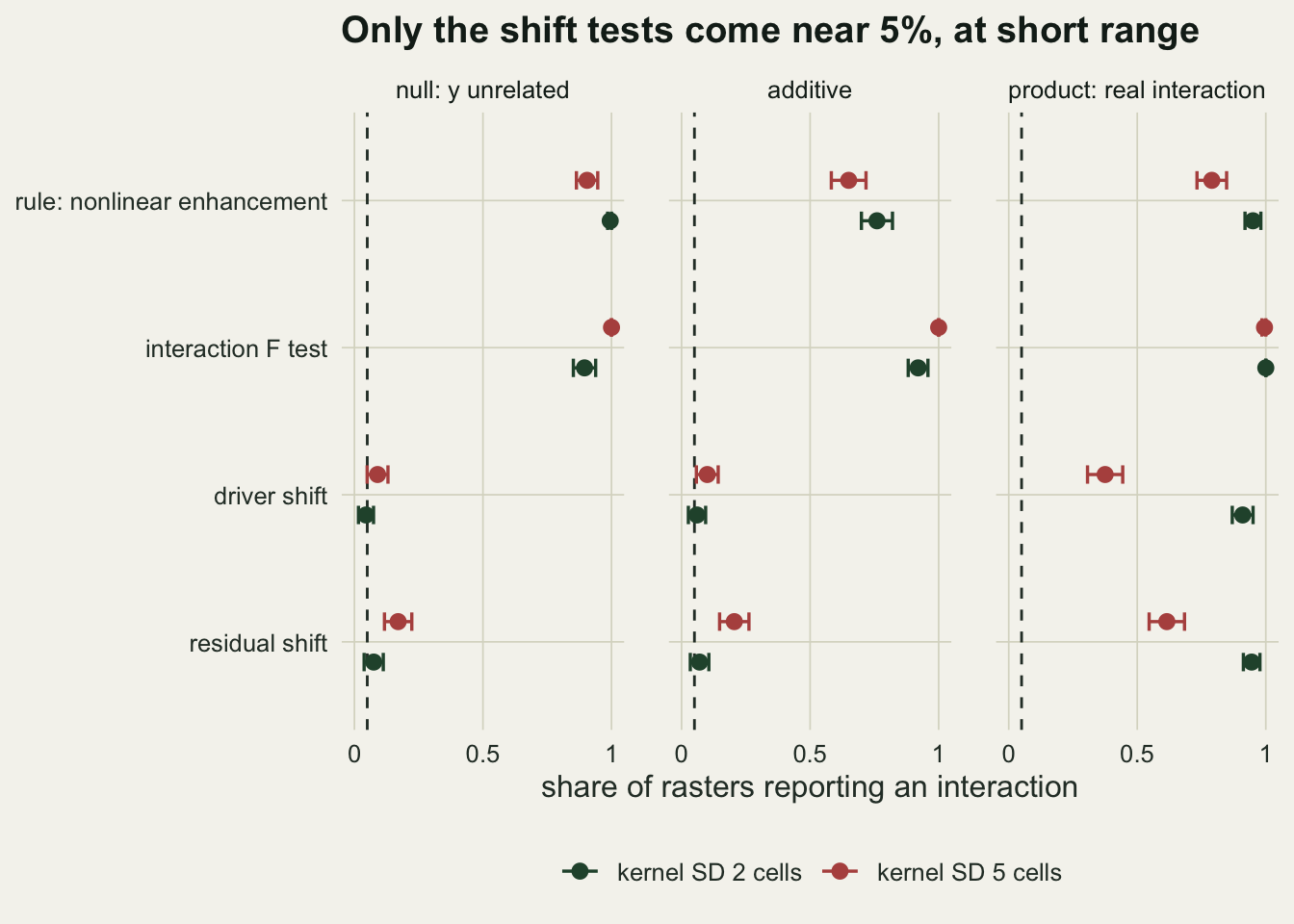

Figure 4: Share of 200 simulated rasters in which each procedure reports an interaction, by scenario and range. The dashed line marks five per cent; bars show plus and minus two Monte Carlo standard errors. Only the product scenario contains a real interaction.

In this design, with b = 0.5 and one range for all three layers, the two shift tests are the only procedures that come near the nominal level, and only at the short range. At a kernel standard deviation of 2 cells the driver shift rejects in 4.5 per cent of null grids and 6.0 per cent of additive ones, and the residual shift in 7.5 and 7.0 per cent; a rate of five per cent has a Monte Carlo standard error of 0.015 here. At 5 cells the driver shift rejects in 9.0 and 10.0 per cent and the residual shift in 17.0 and 20.5 per cent. With the real interaction present, the driver shift finds it in 91.0 per cent of grids at the short range and 37.5 per cent at the long one, and the residual shift in 94.5 and 61.5 per cent.

Part of what goes wrong at the long range is the edge of the map. A toroidal shift wraps the layer round, so the cells that leave one edge come back in at the opposite one, and on a map that does not wrap this puts unrelated values side by side along a seam. When the three layers are generated to wrap exactly at the window’s edges, which no real map does, the driver shift at a kernel standard deviation of 5 cells rejects in 6.0 per cent of null grids and 6.0 per cent of additive ones, and the residual shift in 8.0 and 8.5 per cent. The drop for the residual shift is 2.7 and 3.5 times the standard error of the difference, so on these estimates the seam accounts for most of its excess over five per cent at this range; the drop for the driver shift is 1.1 and 1.5 standard errors, within Monte Carlo error. A real map cannot be made to wrap, so on a real map the long-range rates in the figure are the relevant ones.

The driver shift also rests on a condition that an additive response breaks. Its reference distribution is right only when the shifted layer is independent of the response and of the other driver, and looks the same after the shift as before. In the null scenario that holds apart from the seam. An additive response that depends on x2 breaks it whenever b is not zero: what the shift tests is independence of the x2 layer from the other two, not absence of interaction. Nothing then guarantees its size, and the design above is one case, so two more designs were run, fixed before running, each with 400 additive grids, drivers at a kernel standard deviation of 2 cells and b = 1: the error at the same range, and the error at 5 cells.

mix_grid <- function(r_x, r_e, b) {
  x1 <- smooth_layer(n_side, r_x)
  x2 <- smooth_layer(n_side, r_x)
  e  <- smooth_layer(n_side, r_e)
  y  <- b * x1 + b * x2 + e
  g1 <- disc_q(x1, n_class)
  g2 <- disc_q(x2, n_class)
  f_obs <- f_inter(matrix(y), g1, g2)
  s_id <- sample.int(n_side^2 - 1, n_shift)
  dx <- s_id %/% n_side
  dy <- s_id %% n_side
  f_drv <- vapply(seq_len(n_shift), function(i)
    f_inter(matrix(y), g1, g2[shift_index(n_side, dx[i], dy[i])]), 0)
  x_add <- cbind(1, outer(g1, 2:n_class, "==") + 0, outer(g2, 2:n_class, "==") + 0)
  fit_add <- qr.fitted(qr(x_add), y)
  res_add <- y - fit_add
  y_star <- vapply(seq_len(n_shift), function(i)
    fit_add + res_add[shift_index(n_side, dx[i], dy[i])], numeric(n_side^2))
  c(drv_rej = sum(f_drv >= f_obs) + 1 <= 5,
    res_rej = sum(f_inter(y_star, g1, g2) >= f_obs) + 1 <= 5)
}
mix_set <- data.frame(r_x = c(2, 2), r_e = c(2, 5), b = c(1, 1))
n_mix <- 400
set.seed(4311)
mix_tab <- do.call(rbind, lapply(seq_len(nrow(mix_set)), function(k) {
  out <- t(replicate(n_mix, mix_grid(mix_set$r_x[k], mix_set$r_e[k], mix_set$b[k])))
  data.frame(mix_set[k, ], drv_rej = mean(out[, "drv_rej"]), res_rej = mean(out[, "res_rej"]))
}))
mt <- function(r_e, v) mix_tab[mix_tab$r_e == r_e, v]
mix_se <- sqrt(0.05 * 0.95 / n_mix)
mix_z <- function(r_e, v) (mt(r_e, v) - 0.05) / mix_se
long_drv <- mean(c(gt(5, "null", "drv_rej"), gt(5, "additive", "drv_rej")))
long_drv_z <- (long_drv - 0.05) / sqrt(0.05 * 0.95 / (2 * n_grid_rep))

With the error at the same range as the drivers, the driver shift rejects in 4.8 per cent of grids and the residual shift in 9.0 per cent; with the error at 5 cells, in 7.8 and 12.0 per cent. A rate of five per cent has a Monte Carlo standard error of 0.011 here. The residual shift is too liberal in both designs, by 3.7 and 6.4 standard errors. The driver shift holds with the error at the drivers’ range and sits 2.5 standard errors above five per cent with the longer-range error. On one run that is not decisive; it is also not the guarantee a test needs, since nothing in the method keeps its size near five per cent once the response depends on the shifted layer.

The five verdicts, side by side

set.seed(4308)
prod_raw <- data.frame(t(replicate(n_rep, {
  x1 <- rnorm(n_unit)
  x2 <- rnorm(n_unit)
  gd_pieces(0.5 * x1 + 0.5 * x2 + 0.5 * x1 * x2 + rnorm(n_unit),
            disc_q(x1, n_class), disc_q(x2, n_class))
})))
prod_raw$verdict <- gd_verdict(prod_raw$q1, prod_raw$q2, prod_raw$q12)
prod_enh <- mean(prod_raw$verdict == "enhance, nonlinear")
prod_f   <- mean(prod_raw$f_p < 0.05)

pick <- list(
  "independent units, additive, N 1024" = rate_raw$verdict[rate_raw$n == 1024 & rate_raw$b == 0.5],
  "independent units, additive, N 16384" = rate_raw$verdict[rate_raw$n == 16384 & rate_raw$b == 0.5],
  "correlated drivers r 0.5, additive" = cor_raw$verdict[cor_raw$rho == 0.5],
  "correlated drivers r -0.5, additive" = cor_raw$verdict[cor_raw$rho == -0.5],
  "raster, SD 2 cells, y unrelated" = grid_raw$verdict[grid_raw$r == 2 & grid_raw$scn == "null"],
  "raster, SD 5 cells, additive" = grid_raw$verdict[grid_raw$r == 5 & grid_raw$scn == "additive"],
  "independent units, real interaction" = prod_raw$verdict)
vd_df <- do.call(rbind, lapply(names(pick), function(nm) {
  tb <- table(factor(pick[[nm]], verdict_levels))
  data.frame(scenario = nm, verdict = factor(names(tb), verdict_levels), share = as.numeric(tb) / length(pick[[nm]]))
}))
vd_df$scenario <- factor(vd_df$scenario, rev(names(pick)))
all_q <- rbind(rate_raw[, c("q1", "q2", "q12", "single")], cor_raw[, c("q1", "q2", "q12", "single")],
               grid_raw[, c("q1", "q2", "q12", "single")], wrap_raw[, c("q1", "q2", "q12", "single")],
               prod_raw[, c("q1", "q2", "q12", "single")])
stopifnot(all(all_q$q12 >= pmax(all_q$q1, all_q$q2) - 1e-12))
n_all    <- nrow(all_q)
n_single <- sum(all_q$single > 0)
stopifnot(all(vd_df$share[vd_df$verdict %in% verdict_levels[c(2, 4, 5)]] == 0))

With the real interaction, on independent units, the rule reports a nonlinear enhancement in 100.0 per cent of datasets and the F test rejects in 100.0 per cent. That is the case the verdict is meant for, and the figure puts it next to six cases without any interaction. Across all 10800 datasets simulated in this post, q12 was never below the larger of q1 and q2, so no dataset received either weakening verdict; 85 of them had a combined class holding a single unit, the case in which the GD code would have dropped units.

ggplot(vd_df, aes(share, scenario, fill = verdict)) +
  geom_col(width = 0.7, colour = te_paper, linewidth = 0.3) +
  scale_fill_manual(values = c("enhance, nonlinear" = te_rust, "independent" = te_line,
                               "enhance, bi-" = te_gold, "weaken, uni-" = te_forest,
                               "weaken, nonlinear" = te_ink), drop = FALSE, name = NULL) +
  scale_x_continuous(breaks = c(0, 0.25, 0.5, 0.75, 1), labels = c("0", "0.25", "0.5", "0.75", "1"),
                     expand = expansion(mult = c(0, 0.03))) +
  labs(x = "share of datasets", y = NULL,
       title = "The verdict follows N, correlation and space") +
  theme_datasheet() +
  theme(legend.position = "bottom", panel.grid.major.y = element_blank()) +
  guides(fill = guide_legend(nrow = 2))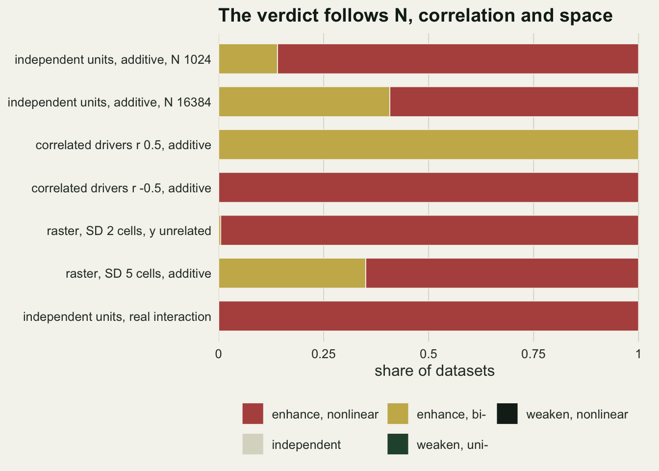

Figure 5: Share of datasets given each of the five interaction types by the rule, for six scenarios with no interaction and one with a real interaction (bottom row). The independent and the two weakening types do not occur.

What to report

Report q for each driver with its number of classes, the number of units, and the expected q of an unrelated classification, (L - 1) / (N - 1). The q of a single driver is a legitimate description of how much of the variance lines up with its classes, and it is the same number as the R-squared of a one-way analysis of variance. Report the q of the combined classes against (L1 L2 - 1) / (N - 1), not against q1 + q2.

Do not use the five interaction types as evidence of interaction. On independent units and additive drivers the verdict was decided by the number of units and the effect size, with correlated drivers by the sign of the correlation between their contributions, and on a raster by the spatial structure. When the question is whether two drivers interact and the units are independent, fit a model on the continuous drivers with an interaction term and test it, as in the spline comparison above. The F test on the classes is safe only while the drivers are close to uncorrelated: the interaction it picks up from correlated drivers belongs to the class means, so its rejection rate grows with the number of units, and at 16384 units a correlation of 0.1 gave 6.0 per cent and one of 0.2 gave 12.8 per cent. Report the correlation between the drivers and the shared fraction q1 + q2 - q_add next to any interaction result.

On a raster or any other spatial layer, report Moran’s I of the response and of the model residuals, and do not trust any F or q test that assumes independent units. Neither spatial test tried here can be recommended. With b = 0.5 and one range for every layer, the toroidal shift of one driver layer came nearest the nominal level: at the short range it rejected in 4.5 and 6.0 per cent of grids without an interaction and found the real one in 91.0 per cent. With b = 1 and an error field of longer range than the drivers it rejected in 7.8 per cent of additive grids. With every layer at the long range it rejected in 9.5 per cent of the null and additive grids taken together, 4.1 standard errors above five per cent, and found the real interaction in only 37.5 per cent. Shifting the residual map instead failed at the long range, 17.0 and 20.5 per cent, and at the short range with b = 1, 9.0 per cent. What a driver shift tests is independence of the shifted layer from the others, not absence of interaction. Any shift test on a real map needs its size checked by simulating layers with the ranges and effect sizes fitted to that map; that step was not tried here, and without it the p value of a shift test is not evidence of interaction.

Honest limits

The simulation uses quantile classes with five classes per driver, and one grid of 32 by 32 cells. The geographical detector literature also uses natural breaks, equal intervals and optimised discretisation, which searches over class counts and break methods for the largest q (Song et al. 2020). A search of that kind raises q1, q2 and q12 by selection and was not simulated. The split into a nonnegative interaction piece and a shared piece holds for any choice of breaks, but the rates here are for quantile classes only.

The drivers are Gaussian and stationary, and the spatial fields are isotropic with a Gaussian kernel. The point-pattern post shows toroidal shift going wrong when both layers follow a shared trend across the plot, and a real elevation layer usually has one; that case was not simulated here, and the shift tests should not be assumed to hold under it. Moran spectral randomisation, the null measured in the map-keeping post, was not tried on the interaction statistic.

Only two ranges and one map size were tried, so how the error rate of the shift tests changes with the ratio of range to map extent is known at two points only. The main spatial run also fixed b = 0.5 and gave the drivers and the error one range; the two extra designs with b = 1 add two points, and four designs do not map out where either test holds. The wrapped-map check shows the seam is part of the long-range problem; it does not say how much of the rest comes from the small number of broad patches a 32 by 32 window holds at that range.

The F test on classes answers a question about class means. With correlated drivers the class means carry a real interaction that the process does not, which is why the spline comparison was run; that comparison assumes the spline basis is flexible enough for the main effects, which holds for the straight lines simulated here and has to be checked for real drivers.

References

Wang JF, Li XH, Christakos G, Liao YL, Zhang T, Gu X, Zheng XY 2010 International Journal of Geographical Information Science 24(1):107-127 (10.1080/13658810802443457)

Wang JF, Zhang TL, Fu BJ 2016 Ecological Indicators 67:250-256 (10.1016/j.ecolind.2016.02.052)

Song Y, Wang J, Ge Y, Xu C 2020 GIScience and Remote Sensing 57(5):593-610 (10.1080/15481603.2020.1760434)

Lotwick HW, Silverman BW 1982 Journal of the Royal Statistical Society Series B 44(3):406-413 (10.1111/j.2517-6161.1982.tb01221.x)

Related tutorials

• Variation partitioning in R: environment vs space
• Interaction terms in ecological GLMs
• Two-species point patterns: testing for interaction
• Permutation nulls that keep the map