library(ggplot2)
library(patchwork)

te_paper  <- "#f5f4ee"
te_ink    <- "#16241d"
te_body   <- "#2c3a31"
te_forest <- "#275139"
te_rust   <- "#b5534e"
te_gold   <- "#c9b458"
te_line   <- "#dad9ca"

theme_datasheet <- function() {
  theme_minimal(base_size = 12) +
    theme(plot.background  = element_rect(fill = te_paper, colour = NA),
          panel.background = element_rect(fill = te_paper, colour = NA),
          panel.grid.major = element_line(colour = te_line, linewidth = 0.3),
          panel.grid.minor = element_blank(),
          text             = element_text(colour = te_body),
          plot.title       = element_text(colour = te_ink, face = "bold"),
          plot.subtitle    = element_text(colour = te_body),
          axis.text        = element_text(colour = te_body))
}Permutation nulls that keep the map
R
spatial
permutation tests
ordination
Procrustes
simulation
ecology tutorial
A site shuffle over-rejects when two maps are smooth. Moran spectral randomisation in R nearly holds its size on a fitted kernel, not on kNN or dbMEM graphs.
Fifty grassland plots, surveyed once for vascular plants and once for ground beetles, and the plot coordinates written in the field book. Each group gets its own ordination, the two configurations are compared with Procrustes, and the question is whether the beetles and the plants order the plots in the same way. The post on comparing two ordinations with Procrustes built that test by hand and then found where it breaks. When both configurations vary smoothly over the same ground, the site shuffle behind PROTEST rejects far more often than it promises, and the post ends its section “Where it stops being calibrated” with the repair named but not run: “A restricted permutation scheme that preserves the spatial arrangement is the repair, and it needs the coordinates, which a bare pair of ordinations does not carry.”
This post runs that repair. The coordinates are in the field book, so the question becomes which map-preserving null to build and what it needs from the analyst. The answer measured below is a decision about the basis. Moran spectral randomisation (MSR) writes a map in an orthogonal set of spatial patterns and randomises the map’s coefficients on those patterns, so every replicate keeps the map’s spatial spectrum. Built from a covariance kernel whose range was fitted to the map, it stays near the nominal five per cent, with one clear excess on a smooth field where the fitted kernel family is wrong. Built from the neighbour graphs that eigenvector methods are usually handed (k nearest neighbours, or the distance-based MEM truncation), it stays liberal in every case simulated here.
None of the method is new. MSR for irregularly spaced sites is Wagner and Dray 2015, whose simulations found correct type I error for correlations between stationary maps “even with very small irregular samples, but was sensitive to linear trend”. Crabot et al. 2019 built the Mantel version. Markello and Misic 2021, comparing ten published null frameworks for brain maps, found that the spatially constrained ones still gave inflated false positive rates when autocorrelation was strong. Bauman et al. 2018 point out that the spatial weighting matrix behind eigenvector methods is usually chosen arbitrarily. Two pieces of what follows are also plain algebra rather than findings: the site shuffle’s rate is predicted, with a modest overestimate, by the effective sample size of Clifford, Richardson and Hemon 1989, and a sign flip on the true kernel is exact by symmetry. Both are derived and then checked. What the simulation adds is the part that is not arithmetic: that a range estimated from the data is good enough, and what the default graphs cost.
Four neighbours set the boundaries. Two-species point patterns uses toroidal shift, the map-keeping null for a rectangle; MSR is the analogue for irregular sites, and it inherits the same weakness to gradients, which gets its own section below. Geographically weighted regression already runs a map-keeping null of another kind, simulating the response from the fitted global model, so a parametric simulation is the rival that MSR has to match here. Moran eigenvector spatial filtering builds the eigenvector maps of a neighbour graph as predictors; here the same eigenvectors carry a null. And the Mantel test post recommends a different repair altogether for spatial confounding, variation partitioning, rather than a constrained null; Crabot et al. 2019 is the null-based counterpart.
The null, written as a sign flip
The statistic is the one from the source post. Centre each two-column configuration and scale it to unit total sum of squares; the Procrustes correlation is the sum of the singular values of \(X^{\top} Y\), which for a \(2 \times 2\) matrix is \(\sqrt{\sum M_{ij}^2 + 2|\det M|}\).
The null keeps \(X\) fixed and randomises \(Y\). Take an orthonormal basis \(V\) of the \(n - 1\) dimensional space of centred maps, the eigenvectors of a doubly centred symmetric matrix: a neighbour graph \(W\) for Moran eigenvector maps, or a covariance kernel \(K\). Every centred map is \(Y = V B\), with coefficients \(B = V^{\top} Y\). Wagner and Dray’s algorithms replace \(B\) by a randomised \(B^{*}\) that keeps the power spectrum (per coefficient for the singleton algorithm, per pair of coefficients for the pair algorithm) and rebuild \(Y^{*} = V B^{*}\). The two used here are the ones in the msr() function of the adespatial package, whose source was read for the definition. The singleton algorithm flips the sign of each coefficient at random, with the same sign for both columns of a configuration, so it keeps the whole spectrum exactly. The pair algorithm, the package default, groups the eigenvectors into consecutive pairs in order of eigenvalue (when their number is odd, one is left out and sign-flipped instead, drawn afresh for every replicate as adespatial does), and turns each pair’s coefficients through a uniform random angle, the same angle for both columns; it keeps the power of each pair. Both are orthogonal maps, so \(Y^{*}\) stays centred with the same sum of squares, and the statistic needs no refit.
Why the choice of \(V\) matters follows in one line. Two independent smooth maps with covariance \(\Sigma\) have centred covariance \(S = H \Sigma H\), with \(H\) the centring matrix, and their coefficients have covariance \(C = V^{\top} S V\). If \(V\) holds the eigenvectors of \(S\) itself, \(C\) is diagonal, the coefficients of a Gaussian map are independent and symmetric about zero, and a sign flip leaves the joint distribution of the data unchanged. The singleton test is then exact by symmetry: its size is 0.05 by construction, and the simulation can only confirm it. Any other basis leaves \(C\) with off-diagonal terms, and flipping signs throws away the correlations between coefficients. That is where the graph bases lose.
r_two_dim <- function(M) sqrt(sum(M^2) + 2 * abs(det(M)))
unit_conf <- function(Z) { Zc <- sweep(Z, 2, colMeans(Z)); Zc / sqrt(sum(Zc^2)) }
r_of <- function(m11, m12, m21, m22)            # vectorised over randomisations
  sqrt(m11^2 + m12^2 + m21^2 + m22^2 + 2 * abs(m11 * m22 - m12 * m21))

kernel_of <- function(D, rng, shape = "exp")
  if (shape == "exp") exp(-D / rng) else exp(-(D / rng)^2)

complement_of <- function(Z) {                   # orthonormal basis orthogonal to the columns of Z
  k <- ncol(Z); qr.Q(qr(cbind(Z, diag(nrow(Z)))))[, (k + 1):nrow(Z)]
}
basis_of <- function(Wmat, Qc) {                 # eigenvectors of Wmat within the space spanned by Qc
  e <- eigen(crossprod(Qc, Wmat %*% Qc), symmetric = TRUE)
  list(V = Qc %*% e$vectors, values = e$values)
}
knn_graph <- function(D, k) {                    # symmetrised k nearest neighbours
  n <- nrow(D); W <- matrix(0, n, n)
  for (i in seq_len(n)) W[i, order(D[i, ])[2:(k + 1)]] <- 1
  pmax(W, t(W))
}
dbmem_graph <- function(D) {                     # distance-based MEM weights, MST threshold
  n <- nrow(D); in_tree <- c(TRUE, rep(FALSE, n - 1)); best <- D[1, ]; thr <- 0
  for (s in 2:n) {
    best[in_tree] <- Inf; j <- which.min(best)
    thr <- max(thr, best[j]); in_tree[j] <- TRUE; best <- pmin(best, D[j, ])
  }
  W <- ifelse(D <= thr, 1 - (D / (4 * thr))^2, 0); diag(W) <- 0; W
}

range_grid <- exp(seq(log(0.02), log(2), length.out = 30))   # extent of the survey is 1
fit_range <- function(Z, D) {                    # profile ML of an exponential range, both columns
  n <- nrow(D); one <- rep(1, n)
  ll <- vapply(range_grid, function(rng) {
    R <- chol(exp(-D / rng) + diag(1e-8, n)); logdet <- 2 * sum(log(diag(R)))
    Ki <- backsolve(R, forwardsolve(t(R), cbind(one, Z)))
    mu <- colSums(Ki[, -1, drop = FALSE]) / sum(Ki[, 1])
    Zr <- sweep(Z, 2, mu); s2 <- colSums(Zr * backsolve(R, forwardsolve(t(R), Zr))) / n
    -0.5 * sum(n * log(s2) + logdet)
  }, 0)
  range_grid[which.max(ll)]
}
fit_range() is what an analyst can do with one map: choose the exponential family, estimate a common mean and variance for each column by generalised least squares, and pick the range with the highest profile likelihood on a grid of thirty values between 0.02 and 2 survey extents. The randomisation is applied to \(Y\), so the range is fitted to \(Y\).
null_singleton <- function(A, B, flips) {        # A = V'X, B = V'Y; one row of flips per replicate
  P <- cbind(A[, 1] * B[, 1], A[, 1] * B[, 2], A[, 2] * B[, 1], A[, 2] * B[, 2])
  M <- flips %*% P
  r_of(M[, 1], M[, 2], M[, 3], M[, 4])
}
null_pair <- function(A, B, angles, left, left_sign) {   # left: the left-out coefficient, one per replicate
  n_pr <- ncol(angles); p <- seq_len(n_pr)
  cross <- function(j, k) list(                  # cross-products of the pairs (j, k), unrotated and rotated
    P = cbind(A[j, 1] * B[j, 1] + A[k, 1] * B[k, 1], A[j, 1] * B[j, 2] + A[k, 1] * B[k, 2],
              A[j, 2] * B[j, 1] + A[k, 2] * B[k, 1], A[j, 2] * B[j, 2] + A[k, 2] * B[k, 2]),
    R = cbind(A[k, 1] * B[j, 1] - A[j, 1] * B[k, 1], A[k, 1] * B[j, 2] - A[j, 1] * B[k, 2],
              A[k, 2] * B[j, 1] - A[j, 2] * B[k, 1], A[k, 2] * B[j, 2] - A[j, 2] * B[k, 2]))
  bef <- cross(2 * p - 1, 2 * p)                 # pair p lies wholly before the left-out coefficient
  Ca <- cos(angles); Sa <- sin(angles)
  if (!length(left)) { M <- Ca %*% bef$P + Sa %*% bef$R; return(r_of(M[, 1], M[, 2], M[, 3], M[, 4])) }
  aft <- cross(2 * p, 2 * p + 1)                 # pair p lies wholly after it
  acr <- cross(2 * p - 1, 2 * p + 1)             # the left-out coefficient sits inside pair p
  w_bef <- outer(left, p, function(l, pp) pp <= (l - 1) %/% 2)
  w_acr <- outer(left, p, function(l, pp) pp == l / 2)
  w_aft <- 1 - w_bef - w_acr
  M <- (Ca * w_bef) %*% bef$P + (Sa * w_bef) %*% bef$R + (Ca * w_aft) %*% aft$P + (Sa * w_aft) %*% aft$R +
    (Ca * w_acr) %*% acr$P + (Sa * w_acr) %*% acr$R +
    left_sign * cbind(A[left, 1] * B[left, 1], A[left, 1] * B[left, 2], A[left, 2] * B[left, 1], A[left, 2] * B[left, 2])
  r_of(M[, 1], M[, 2], M[, 3], M[, 4])
}
p_value <- function(null_r, obs) (1 + sum(null_r >= obs - 1e-12)) / (1 + length(null_r))

set.seed(33101)                                  # check against an explicit rebuild of Y*
n_chk <- 20
xy_chk <- cbind(runif(n_chk), runif(n_chk)); D_chk <- as.matrix(dist(xy_chk))
b_chk <- basis_of(knn_graph(D_chk, 3), complement_of(matrix(1, n_chk)))
X_chk <- unit_conf(matrix(rnorm(2 * n_chk), n_chk)); Y_chk <- unit_conf(matrix(rnorm(2 * n_chk), n_chk))
A_chk <- crossprod(b_chk$V, X_chk); B_chk <- crossprod(b_chk$V, Y_chk); q_chk <- n_chk - 1
fl_chk <- sample(c(-1, 1), q_chk, TRUE)
Y_flip <- b_chk$V %*% (fl_chk * B_chk)
ang_chk <- runif(q_chk %/% 2, 0, 2 * pi); left_chk <- 8L; rot <- diag(q_chk)
pairs_chk <- matrix(setdiff(seq_len(q_chk), left_chk), 2)
for (p in seq_along(ang_chk)) {
  jk <- pairs_chk[, p]
  rot[jk, jk] <- matrix(c(cos(ang_chk[p]), sin(ang_chk[p]), -sin(ang_chk[p]), cos(ang_chk[p])), 2)
}
rot[left_chk, left_chk] <- -1
Y_rot <- b_chk$V %*% rot %*% B_chk
chk_gap <- max(abs(c(r_two_dim(crossprod(X_chk, Y_flip)) - null_singleton(A_chk, B_chk, matrix(fl_chk, 1)),
                     r_two_dim(crossprod(X_chk, Y_rot)) - null_pair(A_chk, B_chk, matrix(ang_chk, 1), left_chk, -1))))
spec_gap <- max(abs(crossprod(b_chk$V, Y_flip)^2 - B_chk^2))
c(largest_gap = chk_gap, spectrum_gap = spec_gap, sum_sq_rebuilt = sum(Y_rot^2))
largest_gap spectrum_gap sum_sq_rebuilt
6.938894e-17 2.053913e-15 1.000000e+00 The vectorised nulls never rebuild \(Y^{*}\); they apply the flips and rotations to the four cross-products directly. Against an explicit rebuild of one flipped and one rotated map, the two routes agree to within floating-point rounding, the flipped map keeps every squared coefficient just as closely (both gaps are printed above), and the rotated map keeps a sum of squares of 1.000000.
What the two kinds of null do to a map is easiest to see on one. The next chunk draws a layout of fifty plots, one smooth configuration from the generator of the source post (an exponential covariance with a range of a quarter of the extent), and one replicate from each null.
set.seed(33102)
n_map <- 50
xy_map <- cbind(runif(n_map), runif(n_map)); D_map <- as.matrix(dist(xy_map))
L_map <- t(chol(kernel_of(D_map, 0.25) + diag(1e-8, n_map)))
Y_map <- unit_conf(L_map %*% matrix(rnorm(2 * n_map), n_map, 2))
rng_map <- fit_range(Y_map, D_map)
V_map <- basis_of(exp(-D_map / rng_map), complement_of(matrix(1, n_map)))$V
Y_shuf <- Y_map[sample.int(n_map), ]
Y_msr <- V_map %*% (sample(c(-1, 1), n_map - 1, TRUE) * crossprod(V_map, Y_map))
nearest <- apply(D_map + diag(Inf, n_map), 1, which.min)
nn_cor <- function(Z) cor(Z[, 1], Z[nearest, 1])
map_cor <- c(observed = nn_cor(Y_map), shuffle = nn_cor(Y_shuf), msr = nn_cor(Y_msr))
round(c(fitted_range = rng_map, map_cor), 3)
fitted_range observed shuffle msr
0.297 0.786 -0.021 0.846 map_df <- rbind(data.frame(x = xy_map[, 1], y = xy_map[, 2], v = Y_map[, 1], what = "observed map"),
data.frame(x = xy_map[, 1], y = xy_map[, 2], v = Y_shuf[, 1], what = "site shuffle"),
data.frame(x = xy_map[, 1], y = xy_map[, 2], v = Y_msr[, 1], what = "sign flip, fitted kernel"))
map_df$what <- factor(map_df$what, levels = c("observed map", "site shuffle", "sign flip, fitted kernel"))
lim <- max(abs(map_df$v))
ggplot(map_df, aes(x, y, fill = v)) +
geom_point(shape = 21, size = 3.4, colour = te_body, stroke = 0.3) +
facet_wrap(~ what) +
coord_fixed() +
scale_fill_gradient2(low = te_forest, mid = te_paper, high = te_rust, limits = c(-lim, lim),
name = "first axis") +
scale_x_continuous(breaks = c(0, 0.5, 1), labels = c("0", "0.5", "1")) +
scale_y_continuous(breaks = c(0, 0.5, 1), labels = c("0", "0.5", "1")) +
labs(x = "easting (survey extent = 1)", y = "northing", title = "Three maps; only the sign flip keeps the spectrum") +
theme_datasheet() +
theme(strip.text = element_text(colour = te_ink, face = "bold"), panel.spacing = unit(1.4, "lines"))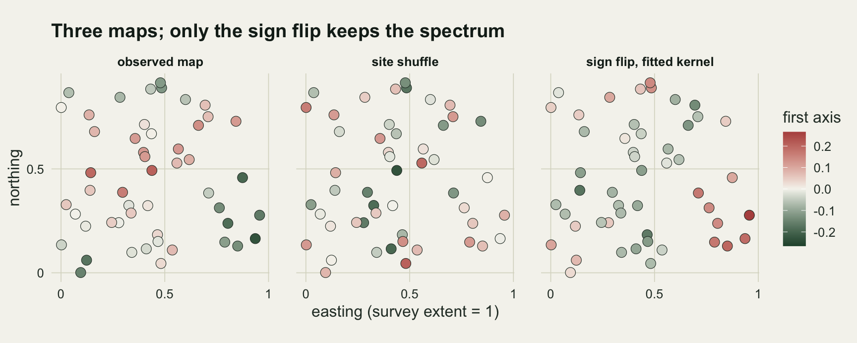
The fitted range for this map is 0.297 against the generating 0.25. The correlation between each plot’s value and its nearest neighbour’s is 0.79 in the observed map, -0.02 after the shuffle and 0.85 after the sign flip. The shuffle builds its null from maps that look nothing like the data, and that is the whole failure the source post measured.
Six nulls, two survey sizes, two kinds of field
The main simulation fixes its design before running. Plots fall uniformly on a unit square, 20 or 50 of them. Each configuration has two independent columns, each a Gaussian field with range 0.25, either with an exponential covariance (rough at short distances, the source post’s generator) or with a Gaussian covariance (smooth). The two configurations of a pair are independent, so every rejection is a false positive. Each cell uses 8 plot layouts and 200 pairs per layout, and every test uses 499 randomisations.
The nulls are the site shuffle and five MSR bases: the true kernel (the symmetry check), the kernel with its range fitted to \(Y\), the distance-based MEM graph truncated at the longest edge of the minimum spanning tree, and symmetric 3 and 6 nearest-neighbour graphs. Each MSR basis runs under both the singleton and the pair algorithm. The fitted kernel is always exponential, including on the Gaussian-covariance fields, where the family is wrong.
n_rand  <- 499
n_lay   <- 8
n_pairs <- 200

run_cell <- function(n, shape, seed) {
  out <- NULL
  for (lay in seq_len(n_lay)) {
    set.seed(seed + lay)
    xy <- cbind(runif(n), runif(n)); D <- as.matrix(dist(xy))
    Sig <- kernel_of(D, 0.25, shape); L <- t(chol(Sig + diag(1e-8, n)))
    Qc <- complement_of(matrix(1, n)); S <- Qc %*% crossprod(Qc, Sig %*% Qc) %*% t(Qc)
    bases <- list(true = basis_of(Sig, Qc), dbmem = basis_of(dbmem_graph(D), Qc),
                  knn3 = basis_of(knn_graph(D, 3), Qc), knn6 = basis_of(knn_graph(D, 6), Qc))
    k_true <- sapply(bases, function(b) {          # variance ratios, see the closed-form section
      Cm <- crossprod(b$V, S %*% b$V); d <- diag(Cm); n_coef <- length(d)
      j <- seq(1, n_coef - 1, 2); k <- j + 1
      c(singleton = sum(Cm^2) / sum(d^2),
        pair = sum(Cm^2) / (sum((d[j] + d[k])^2) / 2 + if (n_coef %% 2) d[n_coef]^2 else 0))
    })
    k_naive <- (n - 1) * sum(S^2) / sum(diag(S))^2
    arms <- c("shuffle", paste(rep(c(names(bases), "fitted"), each = 2), c("singleton", "pair")))
    pv <- matrix(NA, n_pairs, length(arms), dimnames = list(NULL, arms))
    est <- numeric(n_pairs); k_diag <- matrix(NA, n_pairs, 3)
    for (i in seq_len(n_pairs)) {
      X <- unit_conf(L %*% matrix(rnorm(2 * n), n, 2)); Y <- unit_conf(L %*% matrix(rnorm(2 * n), n, 2))
      obs <- r_two_dim(crossprod(X, Y))
      idx <- t(replicate(n_rand, sample.int(n)))
      Y1 <- matrix(Y[idx, 1], n_rand); Y2 <- matrix(Y[idx, 2], n_rand)
      pv[i, "shuffle"] <- p_value(r_of(Y1 %*% X[, 1], Y2 %*% X[, 1], Y1 %*% X[, 2], Y2 %*% X[, 2]), obs)
      flips <- matrix(sample(c(-1, 1), n_rand * (n - 1), TRUE), n_rand)
      angles <- matrix(runif(n_rand * ((n - 1) %/% 2), 0, 2 * pi), n_rand)
      left <- if ((n - 1) %% 2) sample.int(n - 1, n_rand, TRUE) else integer(0)
      left_sign <- sample(c(-1, 1), n_rand, TRUE)
      est[i] <- fit_range(Y, D)
      K_fit <- exp(-D / est[i])
      all_b <- c(bases, list(fitted = basis_of(K_fit, Qc)))
      for (b in names(all_b)) {
        A <- crossprod(all_b[[b]]$V, X); B <- crossprod(all_b[[b]]$V, Y)
        pv[i, paste(b, "singleton")] <- p_value(null_singleton(A, B, flips), obs)
        pv[i, paste(b, "pair")] <- p_value(null_pair(A, B, angles, left, left_sign), obs)
      }
      S_fit <- Qc %*% crossprod(Qc, K_fit %*% Qc) %*% t(Qc)   # the analyst's diagnostic
      k_diag[i, ] <- sapply(bases[2:4], function(b) {
        Cm <- crossprod(b$V, S_fit %*% b$V); sum(Cm^2) / sum(diag(Cm)^2) })
    }
    out <- rbind(out, data.frame(n = n, shape = shape, layout = lay, arm = arms,
                                 rate = colMeans(pv <= 0.05),
                                 k = c(k_naive, as.vector(k_true), NA, NA),
                                 k_fit = c(NA, NA, NA, rep(apply(k_diag, 2, median), each = 2), NA, NA),
                                 range_med = median(est), range_edge = mean(est == max(range_grid))))
  }
  out
}
sweep_res <- rbind(run_cell(20, "exp", 33110), run_cell(50, "exp", 33120),
run_cell(20, "gau", 33130), run_cell(50, "gau", 33140))sweep_res$basis <- sub(" .*", "", sweep_res$arm)
sweep_res$algo <- ifelse(grepl("pair", sweep_res$arm), "pair", "singleton")
cell_sum <- do.call(rbind, lapply(split(sweep_res, list(sweep_res$arm, sweep_res$n, sweep_res$shape)), function(d)
data.frame(n = d$n[1], shape = d$shape[1], arm = d$arm[1], basis = d$basis[1], algo = d$algo[1],
rate = mean(d$rate), med = median(d$rate), lo = min(d$rate), hi = max(d$rate),
se = sd(d$rate) / sqrt(nrow(d)), k = median(d$k), k_fit = median(d$k_fit))))
rt <- function(arm, n, shape, col = "rate") cell_sum[[col]][cell_sum$arm == arm & cell_sum$n == n & cell_sum$shape == shape]
mc_se_layout <- sqrt(0.05 * 0.95 / n_pairs)
graph_arms <- c("dbmem singleton", "knn3 singleton", "knn6 singleton")
exit_fitted <- c(n20 = rt("fitted singleton", 20, "exp", "med"), n50 = rt("fitted singleton", 50, "exp", "med"))
exit_graph <- sapply(graph_arms, rt, n = 50, shape = "exp", col = "med")
range_info <- aggregate(cbind(range_med, range_edge) ~ n + shape, sweep_res[sweep_res$arm == "shuffle", ], median)
f3 <- function(x) sprintf("%.3f", round(x, 3))
pooled_se <- sqrt(0.05 * 0.95 / (n_lay * n_pairs))
fit_pool <- mean(sweep_res$rate[sweep_res$arm == "fitted singleton"]) # all four cells together
true_pool <- mean(sweep_res$rate[sweep_res$arm == "true singleton"])
se_pool <- sqrt(0.05 * 0.95 / (4 * n_lay * n_pairs))
cs_of <- function(basis, algo) cell_sum$rate[cell_sum$basis %in% basis & cell_sum$algo %in% algo]
graph_b <- c("dbmem", "knn3", "knn6")
rough_gap <- max(abs(sapply(c(20, 50), function(n) rt("fitted singleton", n, "exp") - rt("true singleton", n, "exp"))))
g50_smooth <- range(cell_sum$rate[cell_sum$basis %in% graph_b & cell_sum$n == 50 & cell_sum$shape == "gau"])
g_s <- cell_sum[cell_sum$basis %in% graph_b & cell_sum$algo == "singleton", ]
g_p <- cell_sum[cell_sum$basis %in% graph_b & cell_sum$algo == "pair", ]
pair_gap <- max(abs(g_s$rate - g_p$rate[match(paste(g_s$basis, g_s$n, g_s$shape), paste(g_p$basis, g_p$n, g_p$shape))]))
rg <- function(n) range_info$range_med[range_info$n == n & range_info$shape == "exp"]
round(xtabs(rate ~ arm + interaction(n, shape), cell_sum), 3) interaction(n, shape)
arm 20.exp 50.exp 20.gau 50.gau
dbmem pair 0.058 0.081 0.088 0.092
dbmem singleton 0.072 0.071 0.089 0.102
fitted pair 0.052 0.044 0.048 0.061
fitted singleton 0.053 0.046 0.053 0.072
knn3 pair 0.066 0.084 0.100 0.116
knn3 singleton 0.070 0.084 0.106 0.119
knn6 pair 0.083 0.075 0.156 0.100
knn6 singleton 0.091 0.070 0.152 0.099
shuffle 0.224 0.473 0.349 0.694
true pair 0.044 0.044 0.048 0.048
true singleton 0.049 0.048 0.053 0.057round(c(exit_fitted, exit_graph), 3) n20 n50 dbmem singleton knn3 singleton knn6 singleton
0.057 0.048 0.070 0.082 0.075 round(xtabs(med ~ arm + interaction(n, shape), cell_sum[cell_sum$basis == "fitted", ]), 3) # layout medians interaction(n, shape)
arm 20.exp 50.exp 20.gau 50.gau
fitted pair 0.052 0.042 0.048 0.062
fitted singleton 0.057 0.048 0.050 0.070range_info n shape range_med range_edge
1 20 exp 0.1576093 0.000
2 50 exp 0.1847342 0.000
3 20 gau 0.3486658 0.000
4 50 gau 0.6580689 0.005basis_lab <- c(shuffle = "site shuffle", true = "true kernel", fitted = "fitted kernel",
dbmem = "dbMEM graph", knn3 = "3 nearest neighbours", knn6 = "6 nearest neighbours")
cell_lab <- function(n, shape) sprintf("%d plots, %s field", n, ifelse(shape == "exp", "rough", "smooth"))
fig_rates_df <- cell_sum
fig_rates_df$basis_f <- factor(basis_lab[fig_rates_df$basis], levels = rev(basis_lab))
fig_rates_df$cell <- factor(cell_lab(fig_rates_df$n, fig_rates_df$shape),
levels = cell_lab(c(20, 50, 20, 50), c("exp", "exp", "gau", "gau")))
fig_rates_df$algo <- factor(fig_rates_df$algo, levels = c("singleton", "pair"))
p_rates <- ggplot(fig_rates_df, aes(rate, basis_f, colour = algo, shape = algo)) +
geom_vline(xintercept = 0.05, colour = te_ink, linetype = "dashed", linewidth = 0.5) +
geom_errorbar(aes(xmin = lo, xmax = hi), orientation = "y", width = 0, linewidth = 0.6,
position = position_dodge(width = 0.55)) +
geom_point(size = 2.4, stroke = 0.9, fill = te_paper, position = position_dodge(width = 0.55)) +
facet_wrap(~ cell, nrow = 2) +
scale_x_log10(breaks = c(0.03, 0.05, 0.1, 0.2, 0.5), labels = c("0.03", "0.05", "0.1", "0.2", "0.5")) +
scale_colour_manual(values = c(singleton = te_forest, pair = te_rust), name = "MSR algorithm") +
scale_shape_manual(values = c(singleton = 16, pair = 2), name = "MSR algorithm") +
labs(x = "rejection rate of a true null (log scale)", y = NULL,
title = "A fitted kernel stays nearer the level than any graph") +
theme_datasheet() +
theme(legend.position = "bottom", strip.text = element_text(colour = te_ink, face = "bold"))
p_rates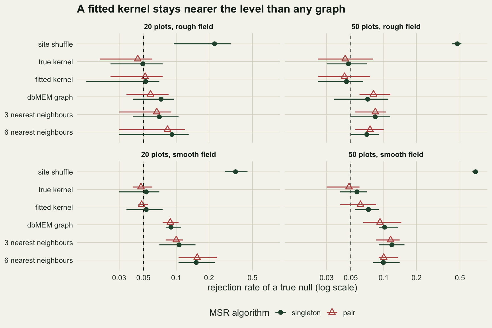
The shuffle rejects 0.224 of the independent pairs at 20 plots on the rough field and 0.473 at 50, and 0.349 and 0.694 on the smooth field. More plots over the same ground add close neighbours rather than independent information, so at a fixed extent the shuffle gets worse as sampling gets denser; the next section shows that this part is arithmetic.
The true kernel, where symmetry settles the answer in advance, gives between 0.048 and 0.057 across the four cells. One layout’s rate carries a Monte Carlo standard error of 0.015 and a cell mean over all 1600 pairs about 0.005, so those four are what an exact test looks like at this replication.
The fitted kernel is the result that is not settled in advance. The range fitted to one configuration is biased low, a median of 0.158 at 20 plots and 0.185 at 50 against the true 0.25, and on the smooth field the exponential family is wrong. The singleton test on that kernel rejects between 0.046 and 0.072 across the cells, and the pair version between 0.044 and 0.061. On the rough field, where the family is right, the singleton flip on the fitted kernel is within 0.003 of the true kernel in both cells, well inside the noise. The one clear excess is the singleton flip on the smooth field at 50 plots, 0.072, about 4 standard errors above 0.05, although still below every graph in that cell (0.092 to 0.119). Pooled over the four cells, the fitted kernel rejects 0.056 against 0.052 for the true kernel, with a pooled standard error of 0.003: estimating the range leaves the test slightly liberal overall, and most of that comes from the one cell where the family is wrong and the plots are many.
The graphs are liberal in every cell and under both algorithms, with rates between 0.058 and 0.156. The worst is the 6-nearest-neighbour graph on the smooth field at 20 plots, 0.152 with the singleton flip. Which graph does worst changes from cell to cell, and so does the effect of sampling density: on the rough field the 3-neighbour graph moves from 0.070 at 20 plots to 0.084 at 50, while the 6-neighbour graph moves from 0.091 to 0.070. Under the singleton flip no graph falls below 0.070 in any cell.
The pair algorithm, the adespatial default, changes little. On the true kernel it gives between 0.044 and 0.048, and on the graphs it differs from the singleton flip by at most 0.014 in any cell. Rotating a pair of coefficients still works inside the graph’s basis, and it cannot restore correlations between coefficients that the basis never separated.
How much of it is arithmetic
Both halves have a formula. Take one entry of the cross-product matrix, \(m = x^{\top} y\) for one column of each configuration, and compare its variance under the process that made the data with its variance under the null.
Under the process, \(x\) and \(y\) are independent with centred covariance \(S\), so \(E(m^2) = \mathrm{tr}(S^2)\). Under the site shuffle, \(m\) has variance \(x^{\top} x \, y^{\top} y / (n - 1)\), whose expectation is \(\mathrm{tr}(S)^2 / (n - 1)\). The ratio
\[k_{\text{shuffle}} = \frac{(n - 1)\,\mathrm{tr}(S^2)}{\mathrm{tr}(S)^2}\]
is the same ratio that Clifford, Richardson and Hemon 1989 use to turn the number of sites into an effective sample size. Under a singleton flip in basis \(V\), \(m = \sum_j A_j B_j\) with \(A = V^{\top} x\) and \(B = V^{\top} y\), and the null variance is \(\sum_j A_j^2 B_j^2\), with expectation \(\sum_j C_{jj}^2\), while the true variance is \(\sum_{j,l} C_{jl}^2\). Their ratio
\[k_{\text{singleton}} = \frac{\sum_{j,l} C_{jl}^2}{\sum_j C_{jj}^2}\]
is one exactly when \(C\) is diagonal and larger otherwise. For the pair rotation the null variance of a pair is \((A_j^2 + A_l^2)(B_j^2 + B_l^2)/2\), with expectation \((C_{jj} + C_{ll})^2 / 2\), which is below \(C_{jj}^2 + C_{ll}^2\) unless the two variances are equal; so the pair version of \(k\) sits slightly above one even on the true kernel, because a rotation mixes two eigenvectors of different variance.
A variance ratio becomes a rejection rate if the four entries are treated as independent normals. The observed statistic is then \(\sqrt{k}\) times a draw of \(r_0\), the Procrustes statistic of a \(2 \times 2\) matrix of independent standard normals, while the null is \(r_0\) itself, and the predicted rate is \(P\{\sqrt{k}\, r_0 > q_{0.95}(r_0)\}\). The chunk takes \(r_0\) from 200 000 draws and \(k\) from the true covariance of each layout, which the sweep chunk stored.
set.seed(33150)
z0 <- matrix(rnorm(8e5), ncol = 4)                # 2e5 draws of a 2 x 2 matrix of iid N(0, 1)
r0 <- sqrt(rowSums(z0^2) + 2 * abs(z0[, 1] * z0[, 4] - z0[, 2] * z0[, 3]))
q95 <- unname(quantile(r0, 0.95))
predicted_rate <- function(k) mean(sqrt(k) * r0 > q95)
pred_df <- cell_sum[!is.na(cell_sum$k), ]
pred_df$pred <- sapply(pred_df$k, predicted_rate)
pred_df$gap <- pred_df$rate - pred_df$pred
pr <- function(arm, n, shape, col = "pred") pred_df[[col]][pred_df$arm == arm & pred_df$n == n & pred_df$shape == shape]
graph_rows <- pred_df$basis %in% c("dbmem", "knn3", "knn6")
gap_rough <- range(pred_df$gap[graph_rows & pred_df$shape == "exp"])
gap_smooth <- range(pred_df$gap[graph_rows & pred_df$shape == "gau"])
excess_ratio_smooth <- (pred_df$rate - 0.05)[graph_rows & pred_df$shape == "gau"] /
  (pred_df$pred - 0.05)[graph_rows & pred_df$shape == "gau"]
k_graph_rng <- range(pred_df$k[graph_rows & pred_df$algo == "singleton"])
k_fit_rng <- range(cell_sum$k_fit, na.rm = TRUE)
shuffle_gap <- range(pred_df$gap[pred_df$basis == "shuffle"])
fit_diag <- pred_df[graph_rows & pred_df$algo == "singleton", ]
fit_diag$pred_fit <- sapply(fit_diag$k_fit, predicted_rate)
fit_below <- sum(fit_diag$pred_fit < fit_diag$rate)
k_rank <- cor(fit_diag$k_fit, fit_diag$rate, method = "spearman")
print(pred_df[, c("n", "shape", "arm", "k", "pred", "rate", "gap")], digits = 3, row.names = FALSE)
n shape arm k pred rate gap
20 exp dbmem pair 1.10 0.0694 0.0581 -0.011320
20 exp dbmem singleton 1.07 0.0639 0.0725 0.008560
20 exp knn3 pair 1.10 0.0693 0.0663 -0.003015
20 exp knn3 singleton 1.07 0.0640 0.0700 0.005950
20 exp knn6 pair 1.16 0.0824 0.0831 0.000730
20 exp knn6 singleton 1.13 0.0748 0.0912 0.016435
20 exp shuffle 1.84 0.2519 0.2244 -0.027530
20 exp true pair 1.02 0.0528 0.0444 -0.008465
20 exp true singleton 1.00 0.0500 0.0494 -0.000625
50 exp dbmem pair 1.19 0.0892 0.0806 -0.008535
50 exp dbmem singleton 1.13 0.0760 0.0713 -0.004710
50 exp knn3 pair 1.22 0.0950 0.0838 -0.011265
50 exp knn3 singleton 1.19 0.0878 0.0838 -0.004020
50 exp knn6 pair 1.14 0.0772 0.0750 -0.002155
50 exp knn6 singleton 1.11 0.0714 0.0700 -0.001430
50 exp shuffle 3.23 0.5379 0.4731 -0.064800
50 exp true pair 1.02 0.0532 0.0444 -0.008845
50 exp true singleton 1.00 0.0500 0.0475 -0.002500
20 gau dbmem pair 1.11 0.0711 0.0881 0.016995
20 gau dbmem singleton 1.09 0.0675 0.0894 0.021885
20 gau knn3 pair 1.14 0.0770 0.1000 0.023040
20 gau knn3 singleton 1.12 0.0738 0.1062 0.032435
20 gau knn6 pair 1.30 0.1144 0.1556 0.041175
20 gau knn6 singleton 1.25 0.1027 0.1525 0.049755
20 gau shuffle 2.34 0.3716 0.3494 -0.022215
20 gau true pair 1.01 0.0523 0.0475 -0.004830
20 gau true singleton 1.00 0.0500 0.0531 0.003125
50 gau dbmem pair 1.16 0.0814 0.0925 0.011070
50 gau dbmem singleton 1.11 0.0721 0.1019 0.029760
50 gau knn3 pair 1.25 0.1028 0.1156 0.012820
50 gau knn3 singleton 1.22 0.0960 0.1187 0.022715
50 gau knn6 pair 1.13 0.0766 0.1000 0.023385
50 gau knn6 singleton 1.11 0.0711 0.0994 0.028270
50 gau shuffle 4.76 0.7098 0.6937 -0.016065
50 gau true pair 1.02 0.0540 0.0481 -0.005910
50 gau true singleton 1.00 0.0500 0.0569 0.006875The prediction for the shuffle is 0.252 and 0.538 on the rough field, against a measured 0.224 and 0.473, and 0.372 and 0.710 on the smooth field, against 0.349 and 0.694. The formula runs high by between 0.016 and 0.065, an approximation error from treating the four entries as independent normals when they are neither, but it carries the whole effect: the shuffle’s error is set by the layout and the covariance, and it can be computed before any randomisation is run.
For the graphs, \(k\) runs from 1.07 to 1.25 under the singleton flip. It cannot fall below one, because the squared entries of \(C\) sum to at least its squared diagonal, so the formula can only ever predict a liberal graph null; what the simulation tests is the size. On the rough field it also predicts the size: measured minus predicted runs from -0.011 to 0.016. On the smooth field it does not. There the measured rate is above the prediction by between 0.011 and 0.050, and the measured excess over 0.05 is 1.2 to 2.4 times the predicted excess.
grp <- ifelse(pred_df$basis == "shuffle", "site shuffle",
       ifelse(pred_df$basis == "true", "true kernel", "neighbour graph"))
pred_df$grp <- factor(grp, levels = c("site shuffle", "true kernel", "neighbour graph"))
pred_df$field <- factor(ifelse(pred_df$shape == "exp", "rough field", "smooth field"))
ggplot(pred_df, aes(pred, rate, colour = grp, shape = field)) +
  geom_abline(slope = 1, intercept = 0, colour = "#9a9a8c", linewidth = 0.5) +
  geom_errorbar(aes(ymin = pmax(rate - 2 * se, 0.02), ymax = rate + 2 * se), width = 0, linewidth = 0.5) +
  geom_point(size = 2.6, stroke = 0.9) +
  scale_x_log10(limits = c(0.03, 0.9), breaks = c(0.05, 0.1, 0.2, 0.5)) +
  scale_y_log10(limits = c(0.03, 0.9), breaks = c(0.05, 0.1, 0.2, 0.5)) +
  scale_colour_manual(values = c(te_gold, te_forest, te_rust), name = NULL) +
  scale_shape_manual(values = c(16, 17), name = NULL) +
  coord_fixed() +
  labs(x = "predicted from k (log scale)", y = "measured (log scale)",
       title = "The formula gets the shuffle, not all of the graph") +
  theme_datasheet() +
  theme(legend.position = "right")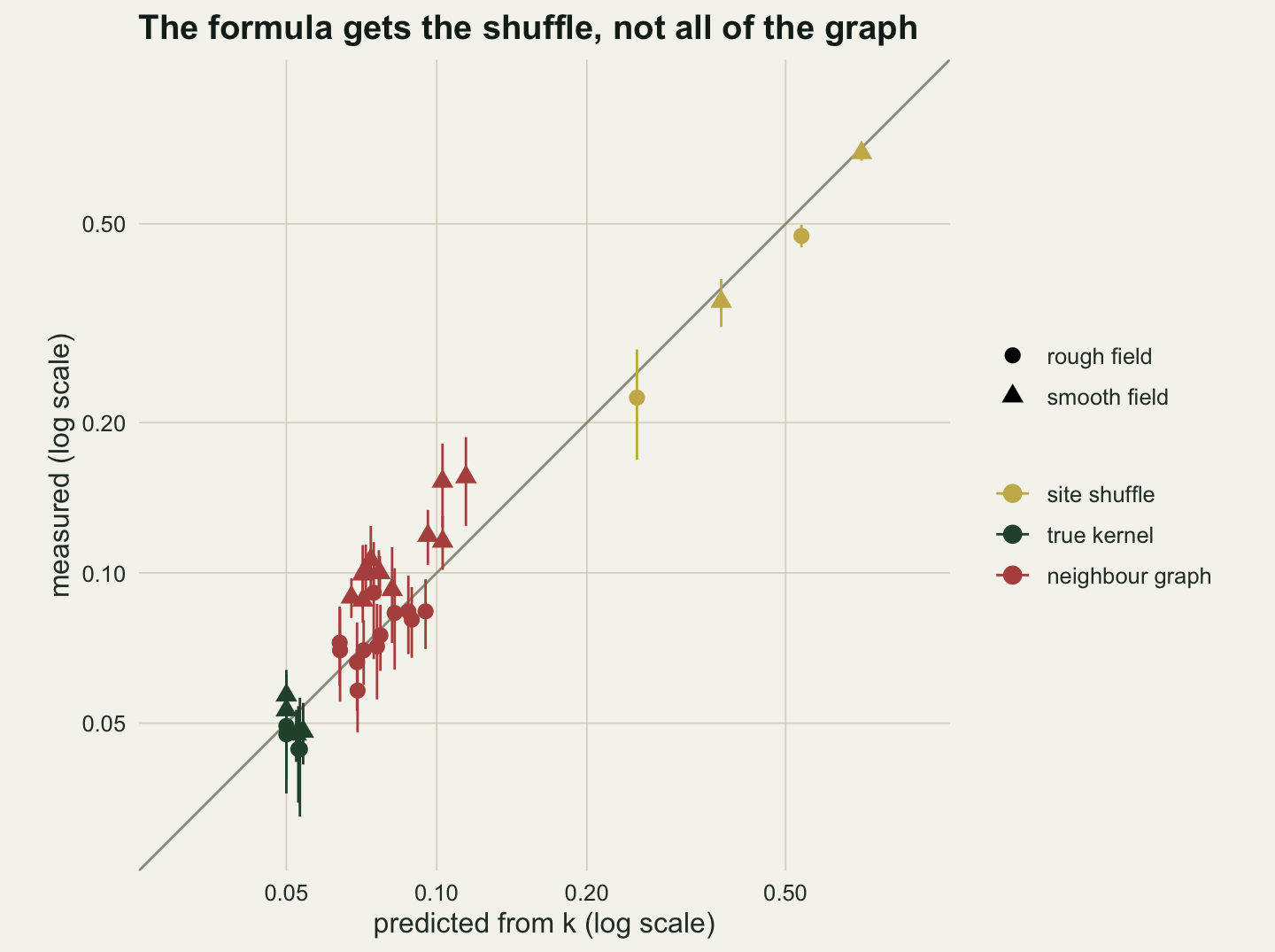
So the shuffle’s rate is arithmetic, and the graph excess is only partly arithmetic. The formula matches the variance of each cross-product and nothing else, and on the smooth field that leaves between 20 and 58 per cent of the graph excess unexplained; that remainder is measured here, not derived.
The formula has a practical use all the same. An analyst does not know \(S\), but can compute \(k\) from the kernel fitted to the map in hand and the graph they intend to use. The sweep chunk did that for every pair. The median of this fitted \(k\) per cell runs from 1.05 to 1.49, never below one, for the same reason. Turned into a rate, it falls below the measured rate in 9 of the 12 graph cells; the exceptions are on the smooth field at 50 plots, where the exponential kernel fitted to a Gaussian-covariance map gives a \(k\) well above the one from the true covariance. Only its size carries information, and loosely: across the 12 graph cells its rank correlation with the measured rate is 0.57, so it is a rough warning, not an estimate.
A fitted kernel against a fitted simulation
The obvious objection is that a map-keeping null does not need eigenvectors at all. The geographically weighted regression post keeps the locations in place and simulates the response from the fitted global model, and the same idea works here: draw Gaussian maps from the fitted exponential kernel and put them in place of \(Y\). It needs the same fitted range as MSR and one Cholesky factor. The two are compared at 30 plots on the rough field, once with Gaussian columns and once with skewed columns, \(\exp(1.2 z)\) of the field, the shape an ordination axis can take when a few abundant species drive it. The 3-nearest-neighbour graph and the shuffle run alongside, over 6 layouts of 150 pairs.
n_riv <- 30; n_lay_riv <- 6; n_pairs_riv <- 150
make_layout <- function(seed, n) {
  set.seed(seed)
  xy <- cbind(runif(n), runif(n)); D <- as.matrix(dist(xy))
  list(xy = xy, D = D, L = t(chol(exp(-D / 0.25) + diag(1e-8, n))),
       Qc = complement_of(matrix(1, n)), knn3 = basis_of(knn_graph(D, 3), complement_of(matrix(1, n)))$V)
}
riv_res <- NULL
for (lay in seq_len(n_lay_riv)) {
  g <- make_layout(33160 + lay, n_riv)
  for (marg in c("Gaussian", "skewed")) {
    tr <- if (marg == "skewed") function(z) exp(1.2 * z) else identity
    pv <- matrix(NA, n_pairs_riv, 4, dimnames = list(NULL, c("shuffle", "fitted", "parametric", "knn3")))
    for (i in seq_len(n_pairs_riv)) {
      X <- unit_conf(tr(g$L %*% matrix(rnorm(2 * n_riv), n_riv, 2)))
      Y <- unit_conf(tr(g$L %*% matrix(rnorm(2 * n_riv), n_riv, 2)))
      obs <- r_two_dim(crossprod(X, Y))
      idx <- t(replicate(n_rand, sample.int(n_riv)))
      Y1 <- matrix(Y[idx, 1], n_rand); Y2 <- matrix(Y[idx, 2], n_rand)
      pv[i, "shuffle"] <- p_value(r_of(Y1 %*% X[, 1], Y2 %*% X[, 1], Y1 %*% X[, 2], Y2 %*% X[, 2]), obs)
      flips <- matrix(sample(c(-1, 1), n_rand * (n_riv - 1), TRUE), n_rand)
      rng_hat <- fit_range(Y, g$D); K_hat <- exp(-g$D / rng_hat)
      V <- basis_of(K_hat, g$Qc)$V
      pv[i, "fitted"] <- p_value(null_singleton(crossprod(V, X), crossprod(V, Y), flips), obs)
      pv[i, "knn3"] <- p_value(null_singleton(crossprod(g$knn3, X), crossprod(g$knn3, Y), flips), obs)
      sims <- t(chol(K_hat + diag(1e-8, n_riv))) %*% matrix(rnorm(n_riv * 2 * n_rand), n_riv)
      sims <- sweep(sims, 2, colMeans(sims)); odd <- seq(1, 2 * n_rand, 2)
      nrm <- sqrt(colSums(sims[, odd]^2) + colSums(sims[, odd + 1]^2))
      CX <- crossprod(sims, X)                     # simulated Gaussian maps replace Y
      pv[i, "parametric"] <- p_value(r_of(CX[odd, 1] / nrm, CX[odd + 1, 1] / nrm,
                                          CX[odd, 2] / nrm, CX[odd + 1, 2] / nrm), obs)
    }
    riv_res <- rbind(riv_res, data.frame(layout = lay, marg = marg, null = colnames(pv), rate = colMeans(pv <= 0.05)))
  }
}
riv_sum <- aggregate(rate ~ marg + null, riv_res, function(v) c(mean = mean(v), lo = min(v), hi = max(v), se = sd(v) / sqrt(length(v))))
riv_sum <- do.call(data.frame, riv_sum)
rv <- function(marg, null, col = "rate.mean") riv_sum[[col]][riv_sum$marg == marg & riv_sum$null == null]
riv_wide <- xtabs(rate ~ interaction(layout, marg) + null, riv_res)
msr_le_param <- sum(riv_wide[, "fitted"] <= riv_wide[, "parametric"])
riv_mc_se <- sqrt(0.05 * 0.95 / (n_lay_riv * n_pairs_riv))
round(xtabs(rate.mean ~ null + marg, riv_sum), 3)
marg
null Gaussian skewed
fitted 0.044 0.050
knn3 0.064 0.064
parametric 0.058 0.071
shuffle 0.328 0.110With Gaussian columns the fitted-kernel MSR rejects 0.044 and the parametric null 0.058; with skewed columns the two give 0.050 and 0.071. MSR is at or below the parametric null in 11 of the 12 layout cells. The Monte Carlo standard error of one of these cell means is 0.007, so the gap on Gaussian columns is within noise and the one on skewed columns is modest. The parametric null is close to the level on Gaussian columns but liberal on skewed ones, about 3 standard errors above 0.05 and no better than the 3-nearest-neighbour graph at the same 30 plots (0.064); the sign flip holds on both. The two differ in one structural way that fits that pattern, although the simulation does not isolate it: the sign flip reuses the observed map’s own coefficients, while the parametric null replaces them with Gaussian draws. On Gaussian columns the 3-nearest-neighbour graph gives 0.064; the shuffle gives 0.328 on Gaussian and 0.110 on skewed columns.
Gradients need their own basis
Wagner and Dray 2015 found MSR sensitive to linear trend, and the point-pattern post found that the toroidal shift fails when both species follow the same gradient. A gradient is not part of a stationary field, so no basis fitted to a stationary kernel can be expected to carry it. The next chunk gives every column of every configuration its own linear gradient in a random direction, with coefficients per unit of extent drawn with standard deviation 1 or 3, on top of the unit-variance field. The two configurations remain independent, so the null is still true; they are no longer stationary.
Two ways of removing the gradient are compared. Both regress each column on the plot coordinates and test the residual configurations. The first then runs MSR on the fitted kernel as before. The second builds the basis inside the space the residuals live in: the eigenvectors of the fitted kernel restricted to the \(n - 3\) dimensions orthogonal to the intercept and the two coordinates, which is what complement_of(H3) supplies.
trend_sd <- c(1, 3)
trd_res <- NULL
for (lay in seq_len(n_lay_riv)) {
  g <- make_layout(33170 + lay, n_riv)
  H3 <- cbind(1, g$xy); Q3 <- complement_of(H3)
  detrend <- function(Z) unit_conf(Z - H3 %*% qr.solve(H3, Z))
  for (s in trend_sd) {
    pv <- matrix(NA, n_pairs_riv, 5, dimnames = list(NULL, c("shuffle", "knn3", "fitted", "detrended", "detrended, residual basis")))
    for (i in seq_len(n_pairs_riv)) {
      X <- g$L %*% matrix(rnorm(2 * n_riv), n_riv, 2) + g$xy %*% matrix(rnorm(4, 0, s), 2)
      Y <- g$L %*% matrix(rnorm(2 * n_riv), n_riv, 2) + g$xy %*% matrix(rnorm(4, 0, s), 2)
      X <- unit_conf(X); Y <- unit_conf(Y); obs <- r_two_dim(crossprod(X, Y))
      idx <- t(replicate(n_rand, sample.int(n_riv)))
      Y1 <- matrix(Y[idx, 1], n_rand); Y2 <- matrix(Y[idx, 2], n_rand)
      pv[i, "shuffle"] <- p_value(r_of(Y1 %*% X[, 1], Y2 %*% X[, 1], Y1 %*% X[, 2], Y2 %*% X[, 2]), obs)
      flips <- matrix(sample(c(-1, 1), n_rand * (n_riv - 1), TRUE), n_rand)
      pv[i, "knn3"] <- p_value(null_singleton(crossprod(g$knn3, X), crossprod(g$knn3, Y), flips), obs)
      V <- basis_of(exp(-g$D / fit_range(Y, g$D)), g$Qc)$V
      pv[i, "fitted"] <- p_value(null_singleton(crossprod(V, X), crossprod(V, Y), flips), obs)
      Xd <- detrend(X); Yd <- detrend(Y); obs_d <- r_two_dim(crossprod(Xd, Yd))
      K_d <- exp(-g$D / fit_range(Yd, g$D))
      Vd <- basis_of(K_d, g$Qc)$V
      pv[i, "detrended"] <- p_value(null_singleton(crossprod(Vd, Xd), crossprod(Vd, Yd), flips), obs_d)
      V3 <- basis_of(K_d, Q3)$V
      pv[i, "detrended, residual basis"] <- p_value(null_singleton(crossprod(V3, Xd), crossprod(V3, Yd),
                                                                   flips[, seq_len(n_riv - 3)]), obs_d)
    }
    trd_res <- rbind(trd_res, data.frame(layout = lay, trend = s, null = colnames(pv), rate = colMeans(pv <= 0.05)))
  }
}
trd_sum <- do.call(data.frame, aggregate(rate ~ trend + null, trd_res,
  function(v) c(mean = mean(v), lo = min(v), hi = max(v))))
td <- function(s, null) trd_sum$rate.mean[trd_sum$trend == s & trd_sum$null == null]
round(xtabs(rate.mean ~ null + trend, trd_sum), 3)
trend
null 1 3
detrended 0.103 0.108
detrended, residual basis 0.058 0.060
fitted 0.053 0.082
knn3 0.079 0.353
shuffle 0.448 0.858Without any detrending, the fitted-kernel MSR rejects 0.053 with the weaker gradient and 0.082 with the stronger one; the 3-nearest-neighbour graph gives 0.079 and 0.353, and the shuffle 0.448 and 0.858. Detrending and then flipping in the full basis is worse than not detrending at both strengths: 0.103 and 0.108. The reason is geometric. The residual configuration \(X_d\) has nothing left along the coordinate directions, but a flip in the full basis spreads the residual \(Y_d\) back over all \(n - 1\) dimensions, so part of every replicate lands where \(X_d\) cannot see it, the replicated statistics come out too small, and the null is too narrow. Built in the residual space, the flips never leave it, and the test gives 0.058 and 0.060.
dep_a <- data.frame(panel = "departure from Gaussian margins", case = riv_sum$marg,
                    null = riv_sum$null, rate = riv_sum$rate.mean, lo = riv_sum$rate.lo, hi = riv_sum$rate.hi)
dep_b <- data.frame(panel = "a random gradient in each map", case = sprintf("gradient SD %d", trd_sum$trend),
                    null = trd_sum$null, rate = trd_sum$rate.mean, lo = trd_sum$rate.lo, hi = trd_sum$rate.hi)
null_lab <- c(shuffle = "site shuffle", knn3 = "3 nearest neighbours", fitted = "fitted kernel",
              parametric = "parametric, fitted field", detrended = "detrended, full basis",
              `detrended, residual basis` = "detrended, residual basis")
dep_plot <- function(d, cols, ttl) {
  d$null_f <- factor(null_lab[d$null], levels = rev(null_lab))
  ggplot(d, aes(rate, null_f, colour = case, shape = case)) +
    geom_vline(xintercept = 0.05, colour = te_ink, linetype = "dashed", linewidth = 0.5) +
    geom_errorbar(aes(xmin = lo, xmax = hi), orientation = "y", width = 0, linewidth = 0.6,
                  position = position_dodge(width = 0.5)) +
    geom_point(size = 2.4, position = position_dodge(width = 0.5)) +
    scale_x_log10(breaks = c(0.03, 0.05, 0.1, 0.2, 0.5, 0.9), labels = c("0.03", "0.05", "0.1", "0.2", "0.5", "0.9")) +
    scale_colour_manual(values = cols, name = NULL) +
    scale_shape_manual(values = c(16, 17), name = NULL) +
    labs(x = "rejection rate (log scale)", y = NULL, title = ttl) +
    theme_datasheet() +
    theme(legend.position = "bottom", plot.title = element_text(size = 11, colour = te_ink, face = "bold"))
}
dep_plot(dep_a, c(te_forest, te_gold), "Gaussian or skewed columns") +
  dep_plot(dep_b, c(te_forest, te_rust), "A gradient in each map") +
  plot_annotation(theme = theme_datasheet())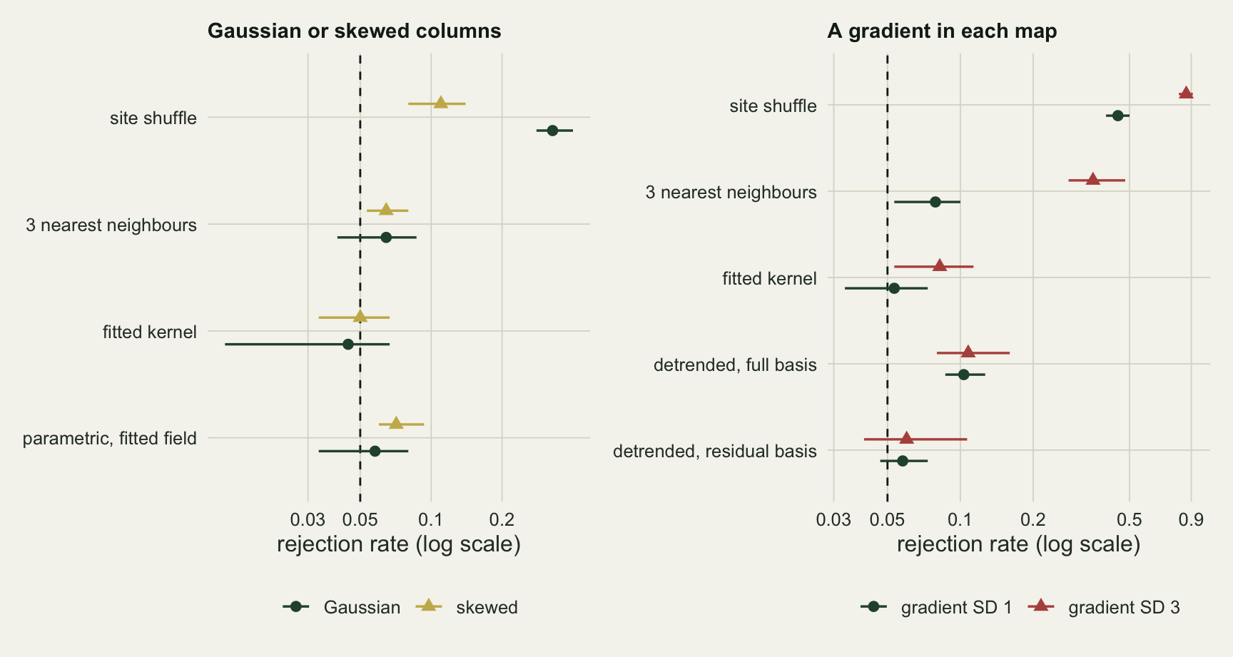
The rule that follows is short: whatever has been fitted out of the data has to be taken out of the randomisation too.
What to report
Report the null alongside the p-value, in enough detail to rebuild it: that it is a Moran spectral randomisation (Wagner and Dray 2015), which basis it used and how that basis was obtained, singleton or pair, and the number of randomisations. The Procrustes correlation and \(m^2\) belong next to it, as the source post argues.
When two maps are sampled at the same plots and the coordinates are known, fit a covariance range to the map you randomise and build the basis from the fitted kernel, doubly centred. In the simulations above that null rejected between 0.044 and 0.072 of independent pairs in the main cells, with the range estimated from 20 or 50 plots. The adespatial msr() function accepts a basis in place of a neighbour list, so the same basis can be handed to it; according to the function’s source it must be an ade4 orthobasis object, with the \(n - 1\) columns scaled to length \(\sqrt{n}\), a weights attribute of rep(1/n, n) and the eigenvalues as its values attribute. The hand-off itself was not run here.
If a neighbour graph is used anyway, compute \(k\) from the fitted kernel and that graph, and report it. It equals one only for a basis that diagonalises the fitted kernel, so a graph basis almost always gives more than one and only the size matters; the graphs here had fitted values of 1.05 to 1.49 and rejected 0.058 to 0.156 of true nulls.
If either map carries a broad gradient, remove it by regression on the coordinates and build the basis in the residual space; detrending and then flipping in the full basis rejected 0.103 and 0.108 here. Say that the test is then about association beyond the gradients, which is a narrower question than association.
Honest limits
Every map here is a Gaussian field with one range and no nugget, the two configurations share one covariance, and the plots are uniform on a square. The fitted kernel was always exponential; on the Gaussian-covariance field at 50 plots it gave the largest fitted-kernel rate in the main simulation, 0.072, still below every graph in that cell. A field with two scales of structure, anisotropy or a measurement nugget was not tried, and a single-range kernel may fit such a map badly. The exactness argument needs the basis to diagonalise the covariance of the randomised map only, so maps with different covariances should be handled by fitting the kernel to the map that is flipped; that case was not simulated.
Real ordination axes are estimated, and a configuration from a spatially structured community is not a Gaussian field. The skewed columns are one step in that direction, not a model of an ordination. The statistic is the Procrustes correlation on two columns; a single Pearson correlation between two mapped variables, for which the Clifford et al. 1989 modified test is the closed-form alternative, and the Mantel version of Crabot et al. 2019 were not run here. Nor was the variogram-matching null of Viladomat et al. 2014, which is a direct rival to MSR on irregular sites.
The gradients were independent between the two maps. A gradient shared by both maps, the case in which the point-pattern post counted toroidal-shift rejections as false positives, was not simulated; whether a test should count it as association is a decision about the question, not about the null. Only the pair and singleton algorithms were implemented; the triplet algorithm in adespatial applies to one variable at a time.
The main cells rest on 8 layouts of 200 pairs, so a cell mean carries a Monte Carlo standard error of about 0.005 from sampling pairs alone, and the spread between layouts, shown as bars in the rate figure, adds to that. Two cell means closer than about 0.015, two standard errors of their difference, are not resolved. The closed forms were checked against these simulations, not against an independent exact computation.
References
Clifford P, Richardson S, Hemon D 1989 Biometrics 45(1):123-134 (10.2307/2532039)
Wagner HH, Dray S 2015 Methods in Ecology and Evolution 6(10):1169-1178 (10.1111/2041-210X.12407)
Bauman D, Drouet T, Fortin M-J, Dray S 2018 Ecology 99(10):2159-2166 (10.1002/ecy.2469)
Crabot J, Clappe S, Dray S, Datry T 2019 Methods in Ecology and Evolution 10(4):532-540 (10.1111/2041-210X.13141)
Viladomat J, Mazumder R, McInturff A, McCauley DJ, Hastie T 2014 Biometrics 70(2):409-418 (10.1111/biom.12139)
Markello RD, Misic B 2021 NeuroImage 236:118052 (10.1016/j.neuroimage.2021.118052)