library(ggplot2)

te_pal <- list(forest = "#275139", green = "#2f8f63", sage = "#93a87f",
               clay = "#b5534e", gold = "#cda23f", line = "#dad9ca",
               ink = "#16241d", paper = "#f5f4ee")

theme_te <- function() {
  theme_minimal(base_size = 12) +
    theme(panel.grid.minor = element_blank(),
          panel.grid.major = element_line(colour = "#e7e6dc"),
          plot.background = element_rect(fill = "#f5f4ee", colour = NA),
          panel.background = element_rect(fill = "#f5f4ee", colour = NA),
          plot.title = element_text(face = "bold", colour = te_pal$ink),
          axis.title = element_text(colour = "#2c3a31"),
          axis.text = element_text(colour = "#2c3a31"))
}Comparing two ordinations with Procrustes
R
ordination
multivariate
vegan
ecology tutorial
Two ordinations of the same sites can look different for no ecological reason. Procrustes rotation and a hand-written PROTEST test, calibrated in base R.
Thirty grassland plots, surveyed twice in the same season: once for vascular plants and once for ground beetles. Two ordinations, printed side by side in the same report. The plant map puts the dry plots on the left and the wet ones on the right; the beetle map puts them top and bottom, and one corner of the plant map is the opposite corner of the beetle map. A reader asks whether the two groups are telling different stories.
They may be. But nothing in that description is evidence of it, because none of what the reader compared is a measurement. An ordination axis has no units, no zero and no preferred direction. The information is in where the sites sit relative to one another; everything else about the picture, the angle it is drawn at, whether it is mirrored, how far apart the extremes are on the page, is an accident of the algorithm and of the starting values it was handed.
So the comparison cannot be a comparison of coordinates. It has to be a comparison of shapes. Take one configuration, allow it to be shifted, rotated, reflected and scaled by a single factor, choose the combination that brings it as close as possible to the other, and look at what is left over. Whatever survives that is a genuine disagreement about which sites are near which; everything the transformation removed was never information. The method is Procrustes analysis, and the ecological version of the test attached to it is PROTEST.
Three earlier posts on this blog have already said the frame is arbitrary and then let it go. Ordination with NMDS in R notes that the sign of an NMDS axis carries no meaning; Model-based unconstrained ordination notes that latent axes are identified only up to rotation and sign, so two runs can look mirrored; Designing an ordination figure notes that you may rotate or reflect a configuration freely without changing the fit. Three correct remarks, each left without a consequence. This post is the consequence. If the frame is arbitrary, then any comparison of two ordinations has to quotient the frame out first, and once it does there is a number, a test for that number, and a way of finding which sites are responsible for it.
The machinery below is written out in base R: a singular value decomposition, a permutation loop and a residual vector per site. It gets calibrated four times, against a rotation of known angle, against vegan, and against its own null distribution twice. Three of those calibrations pass. The fourth finds a common ecological situation in which the test rejects far more often than it promises.
suppressPackageStartupMessages(library(vegan))The solution is one singular value decomposition
Write the two configurations as \(n \times k\) matrices \(X\) and \(Y\), one row per site. We want the orthogonal matrix \(A\), the positive scalar \(c\) and the translation \(t\) that minimise
\[\lVert X - (c\,Y A + \mathbf{1}t^{\top}) \rVert_F^2 .\]
The translation goes first and costs nothing to work out: at the optimum the two clouds share a centroid, so centring each matrix on its own column means removes \(t\) from the problem. With \(X_c\) and \(Y_c\) the centred versions, the objective expands to
\[\lVert X_c \rVert^2 + c^2 \lVert Y_c \rVert^2 - 2c\,\mathrm{tr}(A^{\top} Y_c^{\top} X_c),\]
so for any fixed \(c\) the best \(A\) is whichever orthogonal matrix maximises that trace. Let \(M = X_c^{\top} Y_c\) have singular value decomposition \(M = U \Lambda V^{\top}\). The maximum of the trace is \(\sum_i \lambda_i\), the sum of the singular values, and it is attained at \(A = V U^{\top}\). Differentiating what is left with respect to \(c\) gives the scale as the sum of the singular values divided by the total sum of squares of the configuration being moved. That is the whole method: one decomposition of a \(k \times k\) matrix, which for a two-dimensional or three-dimensional ordination is very small indeed.
The residual has a clean form once both configurations are put on a common footing. Centre each one and divide it by its own root sum of squares, so each has total dispersion one; then the minimised residual sum of squares is
\[m^2 = 1 - \Big( \sum_i \lambda_i \Big)^{\!2}\]
with the singular values now taken from the crossproduct of the two normalised matrices. The quantity \(r = \sum_i \lambda_i\) sits in \([0, 1]\) and is called the Procrustes correlation. It is the number PROTEST tests. The two statistics carry the same information, \(m^2 = 1 - r^2\), and both are worth keeping in view because they compress differently: an \(r\) of 0.9, a value most people would call high, leaves an \(m^2\) of 0.19, so nearly a fifth of the dispersion is still unmatched at that point.
procrustes_fit <- function(target, other) {
  Xc <- sweep(target, 2, colMeans(target))
  Yc <- sweep(other, 2, colMeans(other))
  sv <- svd(t(Xc) %*% Yc)
  A <- sv$v %*% t(sv$u)
  cc <- sum(sv$d) / sum(Yc^2)
  fit <- cc * Yc %*% A
  list(rotation = A, scale = cc, fitted = fit, target = Xc,
       ss = sum((Xc - fit)^2), resid = sqrt(rowSums((Xc - fit)^2)))
}

unit_conf <- function(Z) {
  Zc <- sweep(Z, 2, colMeans(Z))
  Zc / sqrt(sum(Zc^2))
}

proc_r <- function(X, Y) sum(svd(t(unit_conf(X)) %*% unit_conf(Y))$d)
procrustes_fit moves other onto target and keeps the residual vector for each site; proc_r returns the symmetric correlation, which does not care which configuration is named first because normalising both removes the asymmetry the scale factor would introduce.
A rotation of known angle, put back
Before using a piece of arithmetic to make a claim about beetles, point it at a case where the answer is known in advance. Take an arbitrary configuration, rotate it by sixty degrees, scale it by two and a half, shift it across the plane, and hand the pair to the function. It should report a rotation of minus sixty degrees, because it is undoing the one applied, a scale that is the reciprocal of the one applied, and no residual at all. Then do it again with a reflection folded in. A reflection is an orthogonal matrix of determinant minus one and the solution is free to use it, so the residual should again be zero and the determinant of the recovered matrix should flip sign.
set.seed(20260731)
n_cal <- 25
X_cal <- cbind(rnorm(n_cal), rnorm(n_cal))
ang_deg <- 60
ang <- ang_deg * pi / 180
rot_true <- matrix(c(cos(ang), sin(ang), -sin(ang), cos(ang)), 2, 2)
flip <- matrix(c(1, 0, 0, -1), 2, 2)
scale_true <- 2.5
shift <- matrix(rep(c(7, -3), each = n_cal), n_cal, 2)

Y_rot <- scale_true * (X_cal %*% rot_true) + shift
Y_ref <- scale_true * (X_cal %*% rot_true %*% flip) + shift

fit_rot <- procrustes_fit(X_cal, Y_rot)
fit_ref <- procrustes_fit(X_cal, Y_ref)
angle_of <- function(A) atan2(A[2, 1], A[1, 1]) * 180 / pi

cal_ang <- angle_of(fit_rot$rotation)
cal_scale <- fit_rot$scale
print(round(c(sites = n_cal, applied_angle_deg = ang_deg,
              applied_scale = scale_true,
              recovered_angle_deg = cal_ang,
              recovered_scale = cal_scale,
              reciprocal_of_applied = 1 / scale_true), 10))
sites applied_angle_deg applied_scale
25.0 60.0 2.5
recovered_angle_deg recovered_scale reciprocal_of_applied
-60.0 0.4 0.4 print(signif(c(angle_error_deg = abs(cal_ang + ang_deg),
scale_error = abs(cal_scale - 1 / scale_true),
residual_ss_rotation = fit_rot$ss,
residual_ss_reflection = fit_ref$ss), 4)) angle_error_deg scale_error residual_ss_rotation
7.105e-15 1.110e-16 5.289e-30
residual_ss_reflection
1.112e-29 print(round(c(determinant_rotation = det(fit_rot$rotation),
determinant_reflection = det(fit_ref$rotation),
m2_rotation = 1 - proc_r(X_cal, Y_rot)^2,
m2_reflection = 1 - proc_r(X_cal, Y_ref)^2), 12)) determinant_rotation determinant_reflection m2_rotation
1 -1 0
m2_reflection
0 The applied rotation was 60 degrees and the recovered one is -60 degrees, an error of 7.105e-15 degrees. The applied scale was 2.5 and the recovered scale is 0.4, against a reciprocal of 0.4. The residual sum of squares is 5.289e-30, which is machine zero for numbers of this size, and \(m^2\) is 0.
With the reflection added, the determinant of the recovered matrix is -1 instead of 1, and the residual is again 1.112e-29. A mirrored ordination is not a different ordination, and the arithmetic says so without being told. Every claim later in this post is a claim about a residual being small or large, and a residual is only interpretable if the machinery producing it returns zero when it should.
The same answer from an independent implementation
vegan has had procrustes and protest for two decades, written by people who solved the problem their own way. Running both on the same pair checks the implementation rather than the mathematics, and it is cheap.
vp_asym <- vegan::procrustes(X_cal, Y_rot, symmetric = FALSE)
vp_sym <- vegan::procrustes(X_cal, Y_rot, symmetric = TRUE)

set.seed(20260732)
X_chk <- matrix(rnorm(2 * 40), 40, 2)
Y_chk <- X_chk %*% rot_true + matrix(rnorm(2 * 40, 0, 0.5), 40, 2)
hand_chk <- procrustes_fit(X_chk, Y_chk)
vegan_chk <- vegan::procrustes(X_chk, Y_chk, symmetric = FALSE)

print(signif(c(hand_scale = fit_rot$scale, vegan_scale = vp_asym$scale,
               hand_m2 = 1 - proc_r(X_cal, Y_rot)^2, vegan_m2 = vp_sym$ss), 6))
hand_scale vegan_scale hand_m2 vegan_m2
4.00000e-01 4.00000e-01 6.66134e-16 0.00000e+00 print(signif(c(hand_ss = hand_chk$ss, vegan_ss = vegan_chk$ss,
ss_difference = abs(hand_chk$ss - vegan_chk$ss),
hand_r = proc_r(X_chk, Y_chk),
vegan_r = sqrt(1 - vegan::procrustes(X_chk, Y_chk,
symmetric = TRUE)$ss)), 8)) hand_ss vegan_ss ss_difference hand_r vegan_r
1.873679e+01 1.873679e+01 1.421086e-14 8.413901e-01 8.413901e-01 print(signif(c(max_resid_difference =
max(abs(sort(hand_chk$resid) -
sort(residuals(vegan_chk))))), 4))max_resid_difference
0 On a noisy pair of forty sites the hand-written residual sum of squares is 18.736794 and vegan reports 18.736794, a difference of 1.421e-14. The per-site residual lengths agree to 0e+00. Two independent routes to the same numbers, which is the most a check like this can say. From here the hand-written version does the work, because the argument of this post is about what the intermediate quantities look like, and those are easier to see in a list you built.
Two runs of the same NMDS, measured two ways
Now the illusion, on data with some ecology in it. Thirty sites along a single environmental gradient, forty species with Gaussian responses on that gradient, Poisson counts. The dissimilarity is Bray-Curtis, written out rather than called, so the whole path from counts to configuration is visible.
bray_hand <- function(m) {
  n <- nrow(m)
  D <- matrix(0, n, n)
  for (i in seq_len(n)) {
    for (j in seq_len(n)) {
      D[i, j] <- sum(abs(m[i, ] - m[j, ])) / sum(m[i, ] + m[j, ])
    }
  }
  D
}

jaccard_hand <- function(m) {
  b <- m > 0
  n <- nrow(b)
  D <- matrix(0, n, n)
  for (i in seq_len(n)) {
    for (j in seq_len(n)) {
      D[i, j] <- 1 - sum(b[i, ] & b[j, ]) / sum(b[i, ] | b[j, ])
    }
  }
  D
}

sim_comm <- function(n_site, n_sp, seed) {
  set.seed(seed)
  grad <- sort(runif(n_site, 0, 10))
  opt <- runif(n_sp, -1, 11)
  tol <- runif(n_sp, 1, 3)
  amp <- runif(n_sp, 10, 60)
  mu <- outer(grad, seq_len(n_sp),
              function(g, j) amp[j] * exp(-((g - opt[j])^2) / (2 * tol[j]^2)))
  m <- matrix(rpois(length(mu), mu), nrow = n_site)
  list(comm = m[, colSums(m) > 0, drop = FALSE], grad = grad)
}

cm <- sim_comm(30, 40, 4242)
D_bray <- bray_hand(cm$comm)
D_jacc <- jaccard_hand(cm$comm)
n_site <- nrow(cm$comm)

dist_check <- max(abs(D_bray - as.matrix(vegdist(cm$comm, "bray"))),
                  abs(D_jacc - as.matrix(vegdist(cm$comm, "jaccard",
                                                 binary = TRUE))))
print(round(c(sites = n_site, species_kept = ncol(cm$comm),
              mean_bray = mean(D_bray[lower.tri(D_bray)]),
              mean_jaccard = mean(D_jacc[lower.tri(D_jacc)])), 4))
sites species_kept mean_bray mean_jaccard
30.0000 40.0000 0.5060 0.3765 print(signif(c(largest_disagreement_with_vegdist = dist_check), 4))largest_disagreement_with_vegdist
1.11e-16 The hand-written matrices reproduce vegdist to 1.11e-16, so the input to the ordination is not in question.
Non-metric multidimensional scaling starts from a configuration and improves it, and the stress function it minimises is invariant to rotation. Two runs from different starting points that reach the same stress have found the same shape in different frames. vegan knows this: both metaMDS and monoMDS rotate their output to principal components by default, so that repeated runs look comparable. Turning that off with pc = FALSE exposes the raw output, which is what an ordination delivers before anyone tidies it. Forty random starts, then the two comparisons the reader in the opening paragraph might make.
n_start <- 40
confs <- vector("list", n_start)
stress_v <- numeric(n_start)
for (s in seq_len(n_start)) {
  set.seed(s)
  y0 <- matrix(rnorm(n_site * 2), n_site, 2)
  nn <- monoMDS(as.dist(D_bray), y = y0, model = "global", pc = FALSE)
  confs[[s]] <- nn$points
  stress_v[s] <- nn$stress
}

same_stress <- which(stress_v < min(stress_v) + 0.001)
ref_conf <- confs[[same_stress[1]]]
cmp <- t(vapply(same_stress, function(i) {
  Ci <- confs[[i]]
  c(cor1 = cor(ref_conf[, 1], Ci[, 1]),
    cor2 = cor(ref_conf[, 2], Ci[, 2]),
    m2 = 1 - proc_r(ref_conf, Ci)^2)
}, numeric(3)))

n_same <- length(same_stress)
print(round(c(starts = n_start, runs_at_same_stress = n_same,
              lowest_stress = min(stress_v),
              highest_stress_kept = max(stress_v[same_stress])), 5))
starts runs_at_same_stress lowest_stress highest_stress_kept
40.00000 18.00000 0.01899 0.01997 print(round(c(cor_axis1_min = min(cmp[, "cor1"]),
cor_axis1_max = max(cmp[, "cor1"]),
cor_axis2_min = min(cmp[, "cor2"]),
cor_axis2_max = max(cmp[, "cor2"]),
cor_axis1_smallest_abs = min(abs(cmp[, "cor1"]))), 4)) cor_axis1_min cor_axis1_max cor_axis2_min
-0.9472 1.0000 -0.9511
cor_axis2_max cor_axis1_smallest_abs
1.0000 0.1902 print(signif(c(m2_min = min(cmp[, "m2"]), m2_max = max(cmp[, "m2"]),
m2_median = median(cmp[, "m2"]),
r_min = min(sqrt(1 - cmp[, "m2"]))), 4)) m2_min m2_max m2_median r_min
4.441e-16 5.934e-03 3.219e-04 9.970e-01 Of 40 random starts, 18 reached a stress within one thousandth of the best value, so those 18 runs agree about the arrangement of the sites to whatever precision the stress function can resolve. Compared axis by axis they do not look like it. The correlation between the reference run’s first axis and the other runs’ first axes runs from -0.9472 to 1, with a smallest absolute value of 0.1902, which is a correlation you would describe as no relationship at all. The second axis behaves the same way, from -0.9511 to 1.
Now the other number for the same 18 pairs. The largest Procrustes \(m^2\) among them is 0.005934, the median is 0.0003219, and the smallest Procrustes correlation is 0.997: less than one per cent of the dispersion fails to superimpose in the worst case.
An axis correlation as low as 0.1902 and an \(m^2\) of at most 0.005934, out of the same set of pairs. The first number is an artefact of the coordinate frame; the second is the answer to the question anyone actually meant to ask.
pick <- same_stress[which.min(abs(cmp[, "cor1"]))]
conf_b <- confs[[pick]]
sup <- procrustes_fit(ref_conf, conf_b)

raw_df <- rbind(
  data.frame(x = ref_conf[, 1], y = ref_conf[, 2], run = "first run",
             panel = "raw coordinates"),
  data.frame(x = conf_b[, 1], y = conf_b[, 2], run = "second run",
             panel = "raw coordinates"),
  data.frame(x = sup$target[, 1], y = sup$target[, 2], run = "first run",
             panel = "after Procrustes"),
  data.frame(x = sup$fitted[, 1], y = sup$fitted[, 2], run = "second run",
             panel = "after Procrustes"))
raw_df$panel <- factor(raw_df$panel,
                       levels = c("raw coordinates", "after Procrustes"))

ggplot(raw_df, aes(x, y, colour = run, shape = run)) +
  geom_point(size = 2.2, alpha = 0.9) +
  facet_wrap(~panel, nrow = 1) +
  coord_fixed() +
  scale_colour_manual(values = c(te_pal$forest, te_pal$clay), name = NULL) +
  scale_shape_manual(values = c(16, 17), name = NULL) +
  labs(x = "first ordination axis", y = "second ordination axis",
       title = "One shape, two frames") +
  theme_te() +
  theme(legend.position = "bottom", plot.margin = margin(8, 14, 4, 8))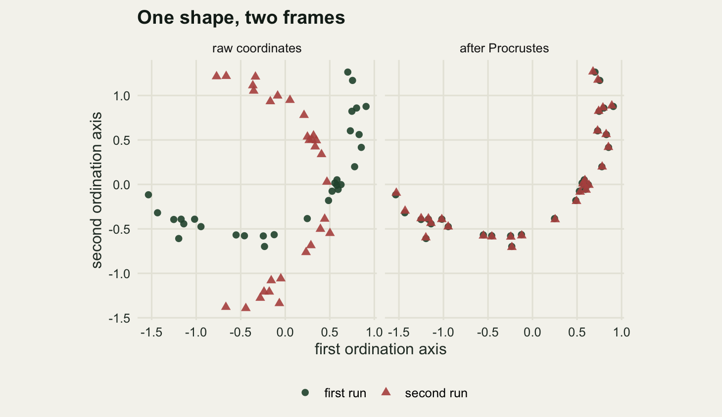
The two panels are the same data. Anyone who compared the left panel and concluded that the two runs had found different community structure would be describing the random number generator that produced the starting configurations.
A permutation test written out
A Procrustes correlation of 0.997 is obviously high, and a correlation of 0.2 would obviously be low, but most real comparisons land in between and the eye is no use there. The null hypothesis worth testing is that the two configurations describe unrelated arrangements of the same sites, and the way to build its distribution is to break the correspondence between rows while leaving both configurations otherwise intact. Permute the site labels of one of them, refit, and record the correlation. That is Jackson’s PROTEST.
Two details make the loop cheap. Permuting rows changes neither the column means nor the total sum of squares, so both configurations can be centred and normalised once, outside the loop. And in two dimensions the sum of the singular values of a \(2 \times 2\) matrix has a closed form: with \(s_1^2 + s_2^2 = \sum M_{ij}^2\) and \(s_1 s_2 = |\det M|\), the sum is \(\sqrt{\sum M_{ij}^2 + 2|\det M|}\), so no decomposition is needed at all.
r_two_dim <- function(M) sqrt(sum(M^2) + 2 * abs(det(M)))

protest_hand <- function(X, Y, nperm = 4999, seed = 1) {
  Xn <- unit_conf(X)
  Yn <- unit_conf(Y)
  n <- nrow(Xn)
  r_obs <- sum(svd(t(Xn) %*% Yn)$d)
  set.seed(seed)
  r_perm <- numeric(nperm)
  for (b in seq_len(nperm)) {
    r_perm[b] <- r_two_dim(t(Xn) %*% Yn[sample.int(n), , drop = FALSE])
  }
  list(r = r_obs, m2 = 1 - r_obs^2, perm = r_perm, nperm = nperm,
       p = (1 + sum(r_perm >= r_obs)) / (1 + nperm))
}

set.seed(20260733)
M_test <- matrix(rnorm(4), 2, 2)
print(signif(c(sum_of_singular_values = sum(svd(M_test)$d),
               closed_form = r_two_dim(M_test),
               difference = abs(sum(svd(M_test)$d) -
                                  r_two_dim(M_test))), 6))
sum_of_singular_values closed_form difference
2.69336e+00 2.69336e+00 4.44089e-16 The closed form agrees with svd to 4.44e-16, so the shortcut is a shortcut and not an approximation.
The first application is an ecological question rather than an algorithmic one: does the choice of dissimilarity index change the map? The same thirty sites, ordinated by principal coordinates on Bray-Curtis and on binary Jaccard, which throws the abundances away. Choosing a dissimilarity index covers what that choice does to the distances; here it is a question about the configurations.
pco_bray <- cmdscale(as.dist(D_bray), k = 2)
pco_jacc <- cmdscale(as.dist(D_jacc), k = 2)

idx <- protest_hand(pco_bray, pco_jacc, nperm = 4999, seed = 20260734)
set.seed(20260734)
idx_vegan <- vegan::protest(pco_bray, pco_jacc, permutations = 4999)

print(round(c(sites = n_site,
              axis1_correlation = cor(pco_bray[, 1], pco_jacc[, 1]),
              axis2_correlation = cor(pco_bray[, 2], pco_jacc[, 2])), 4))
sites axis1_correlation axis2_correlation
30.0000 0.9926 -0.8851 print(signif(c(procrustes_r = idx$r, m2 = idx$m2,
permutations = idx$nperm, p_value = idx$p,
null_mean_r = mean(idx$perm),
null_q95_r = unname(quantile(idx$perm, 0.95)),
max_null_r = max(idx$perm)), 5))procrustes_r m2 permutations p_value null_mean_r null_q95_r
9.6934e-01 6.0374e-02 4.9990e+03 2.0000e-04 1.8945e-01 3.4367e-01
max_null_r
6.1112e-01 print(signif(c(vegan_r = idx_vegan$t0, vegan_p = idx_vegan$signif,
r_difference = abs(idx$r - idx_vegan$t0)), 6)) vegan_r vegan_p r_difference
9.69343e-01 2.00000e-04 1.11022e-16 The two indices give configurations with a Procrustes correlation of 0.9693, an \(m^2\) of 0.0604, and a p-value of 0.0002 from 4999 permutations, the smallest the test can return. Under the null the mean correlation is 0.1894 and the largest permuted value is 0.6111, nowhere near the observed one. vegan::protest returns 0.969343 for the same statistic, differing from the hand-written value by 1.11e-16.
The per-axis correlations tell the usual half-truth: 0.9926 on the first axis and -0.8851 on the second. The sign on the second axis flipped, which means nothing, but the two magnitudes bracket the Procrustes correlation: the first axis agrees more closely than the summary statistic and the second less closely, so what disagreement there is sits mostly on the second, minor axis.
An \(m^2\) of 0.0604 is the honest summary: on this dataset, with a strong single gradient and reasonably complete sampling, discarding the abundances costs about 6 per cent of the configuration. It would not be that small on a dataset where the abundances carry the gradient and the species lists do not.
Does the test hold its size
A p-value is a promise about long-run behaviour, and a permutation test assembled by hand is a good candidate for a broken promise. The check is direct: generate pairs of configurations that are independent by construction, run the test on each, and count how often it rejects at the nominal level.
type_one_run <- function(nrep, nperm, gen, seed) {
  set.seed(seed)
  pv <- numeric(nrep)
  for (i in seq_len(nrep)) {
    Xi <- unit_conf(gen())
    Yi <- unit_conf(gen())
    n_pts <- nrow(Xi)
    r_o <- r_two_dim(t(Xi) %*% Yi)
    hit <- 0L
    for (b in seq_len(nperm)) {
      if (r_two_dim(t(Xi) %*% Yi[sample.int(n_pts), , drop = FALSE]) >= r_o) {
        hit <- hit + 1L
      }
    }
    pv[i] <- (1 + hit) / (1 + nperm)
  }
  pv
}

n_rep <- 1000
n_perm_cal <- 999
n_cal_pts <- 20
gen_iid <- function() matrix(rnorm(n_cal_pts * 2), n_cal_pts, 2)
p_clean <- type_one_run(n_rep, n_perm_cal, gen_iid, 20260735)
mc_se <- sqrt(0.05 * 0.95 / n_rep)

print(c(replicates = n_rep, permutations_each = n_perm_cal,
        sites = n_cal_pts))
replicates permutations_each sites
1000 999 20 print(round(c(rate_at_10 = mean(p_clean <= 0.10),
rate_at_05 = mean(p_clean <= 0.05),
rate_at_01 = mean(p_clean <= 0.01),
monte_carlo_se_at_05 = mc_se,
deviation_in_se = (mean(p_clean <= 0.05) - 0.05) / mc_se), 4)) rate_at_10 rate_at_05 rate_at_01
0.1090 0.0580 0.0070
monte_carlo_se_at_05 deviation_in_se
0.0069 1.1608 print(round(c(mean_p = mean(p_clean), median_p = median(p_clean)), 4)) mean_p median_p
0.4936 0.4840 Over 1000 independent pairs of configurations on 20 sites, each tested with 999 permutations, the test rejected at the nominal five per cent level 5.8 per cent of the time. The Monte Carlo standard error on that estimate is 0.0069, so the observed rate is 1.16 standard errors from nominal. At the ten per cent level the rate is 10.9 per cent and at one per cent it is 0.7 per cent. The mean p-value is 0.4936, which is what a uniform distribution gives.
The test is calibrated. That is the expected result, and still worth the compute, because the next one is not.
Where it stops being calibrated
Permuting site labels assumes the sites are exchangeable under the null, and ecological sites usually are not. Sites near each other tend to resemble each other, in the plants and in the beetles and in anything else measured on them, and that resemblance can come from shared spatial structure alone rather than from any link between the two groups. The test below keeps the two configurations independent, as before, but generates each one as a smooth spatial field over the same site coordinates: an exponential covariance with a range of a quarter of the study extent, unremarkable for a grassland survey.
set.seed(20260736)
site_xy <- cbind(runif(n_cal_pts), runif(n_cal_pts))
cov_range <- 0.25
Sigma <- exp(-as.matrix(dist(site_xy)) / cov_range)
L_chol <- chol(Sigma + diag(1e-8, n_cal_pts))
gen_field <- function() {
  cbind(as.vector(t(L_chol) %*% rnorm(n_cal_pts)),
        as.vector(t(L_chol) %*% rnorm(n_cal_pts)))
}

p_spatial <- type_one_run(n_rep, n_perm_cal, gen_field, 20260737)
print(round(c(sites = n_cal_pts, covariance_range = cov_range,
              replicates = n_rep, permutations_each = n_perm_cal), 4))
sites covariance_range replicates permutations_each
20.00 0.25 1000.00 999.00 print(round(c(rate_at_10 = mean(p_spatial <= 0.10),
rate_at_05 = mean(p_spatial <= 0.05),
rate_at_01 = mean(p_spatial <= 0.01),
inflation_at_05 = mean(p_spatial <= 0.05) / 0.05,
mean_p = mean(p_spatial)), 4)) rate_at_10 rate_at_05 rate_at_01 inflation_at_05 mean_p
0.303 0.213 0.092 4.260 0.314 The rejection rate at the nominal five per cent level is 21.3 per cent, an inflation factor of 4.26. At the one per cent level the rate is 9.2 per cent, an inflation of 9.2. The two fields were drawn independently. Every one of those rejections is a false positive, produced by nothing but the fact that both configurations vary smoothly over the same ground.
This is the same failure that makes Mantel tests over-reject on spatially structured data, and it arrives here through the same door: the permutation scheme, not the statistic. The statistic is fine. What is wrong is the null distribution it gets compared against, because a randomly permuted assignment of sites destroys spatial structure that the observed data has, which makes the observed correlation look extreme against a null it was never drawn from. A restricted permutation scheme that preserves the spatial arrangement is the repair, and it needs the coordinates, which a bare pair of ordinations does not carry.
ecdf_grid <- seq(0, 1, length.out = 201)
ecdf_df <- rbind(
  data.frame(alpha = ecdf_grid, rate = ecdf(p_clean)(ecdf_grid),
             null = "exchangeable sites"),
  data.frame(alpha = ecdf_grid, rate = ecdf(p_spatial)(ecdf_grid),
             null = "spatially smooth sites"))

ggplot(ecdf_df, aes(alpha, rate, colour = null, linetype = null)) +
  geom_abline(slope = 1, intercept = 0, colour = "#9a9a8c",
              linewidth = 0.5) +
  geom_line(linewidth = 0.9) +
  scale_colour_manual(values = c(te_pal$forest, te_pal$clay), name = NULL) +
  scale_linetype_manual(values = c("solid", "22"), name = NULL) +
  labs(x = "nominal level of the test",
       y = "proportion of tests rejecting",
       title = "Where the permutation null stops being the right null") +
  theme_te() +
  theme(legend.position = "bottom", plot.margin = margin(8, 14, 4, 8))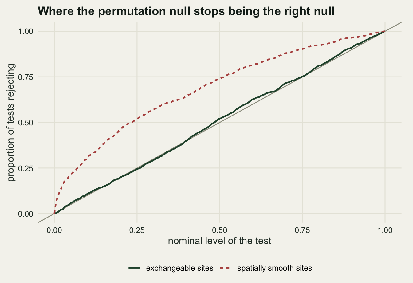
The residuals know things the summary does not
\(m^2\) is one number for a whole survey, and one number can be produced in more than one way. A configuration that has drifted a little everywhere and one that is identical except for two plots can give the same total. The residual vector for site \(i\), the distance between where the site sits in the target and where the superimposed configuration puts it, tells them apart, and it is already in the fit object. Here is a constructed case: thirty sites, a rotation, a scale change, a little noise everywhere, and then two sites shoved a long way.
set.seed(20260738)
n_res <- 30
X_res <- cbind(rnorm(n_res), rnorm(n_res, 0, 0.6))
ang_res <- 0.9
rot_res <- matrix(c(cos(ang_res), sin(ang_res), -sin(ang_res), cos(ang_res)),
                  2, 2)
Y_res <- 1.4 * X_res %*% rot_res + matrix(rnorm(2 * n_res, 0, 0.09), n_res, 2)
moved <- c(7, 22)
Y_res[moved, ] <- Y_res[moved, ] +
  matrix(c(1.5, -1.4, -1.3, 1.6), 2, 2, byrow = TRUE)

fit_res <- procrustes_fit(X_res, Y_res)
r_res <- proc_r(X_res, Y_res)
sq <- fit_res$resid^2
share <- sum(sq[moved]) / sum(sq)
r_drop <- proc_r(X_res[-moved, ], Y_res[-moved, ])
pt_res <- protest_hand(X_res, Y_res, nperm = 4999, seed = 20260739)

print(round(c(sites = n_res, sites_displaced = length(moved),
              procrustes_r = r_res, m2 = 1 - r_res^2,
              p_value = pt_res$p), 5))
sites sites_displaced procrustes_r m2 p_value
30.00000 2.00000 0.96471 0.06934 0.00020 print(round(c(share_of_residual_from_two = share,
even_share_would_be = length(moved) / n_res,
concentration_ratio = share / (length(moved) / n_res)), 4))share_of_residual_from_two even_share_would_be
0.8041 0.0667
concentration_ratio
12.0616 print(round(c(resid_site_7 = fit_res$resid[moved[1]],
resid_site_22 = fit_res$resid[moved[2]],
median_resid = median(fit_res$resid),
largest_over_median =
max(fit_res$resid[moved]) / median(fit_res$resid)), 4)) resid_site_7 resid_site_22 median_resid largest_over_median
1.4179 0.8724 0.1226 11.5656 print(round(c(r_with_all_sites = r_res, r_without_the_two = r_drop,
m2_with_all = 1 - r_res^2, m2_without_the_two = 1 - r_drop^2,
m2_ratio = (1 - r_res^2) / (1 - r_drop^2)), 5)) r_with_all_sites r_without_the_two m2_with_all m2_without_the_two
0.96471 0.99696 0.06934 0.00606
m2_ratio
11.43791 The global summary looks like a good match that is not perfect: a Procrustes correlation of 0.9647, an \(m^2\) of 0.0693, and a p-value of 0.0002. Written into a results section that reads as two configurations broadly agreeing, with some scatter. That is not what the residuals show. Two of the 30 sites carry 80.4 per cent of the residual sum of squares. If the disagreement were spread evenly those two would carry 6.7 per cent, so they are concentrated by a factor of 12.1. Their residual lengths are 1.4179 and 0.8724 against a median of 0.1226 across all sites.
Drop the two and refit: the correlation goes from 0.9647 to 0.997, and \(m^2\) from 0.0693 to 0.00606, a factor of 11.4. The other twenty-eight sites agree almost exactly. The correct sentence is not that the two ordinations broadly agree; it is that they agree everywhere except at sites 7 and 22, and that those two are worth going back to the field notes for.
arr <- data.frame(x0 = fit_res$target[, 1], y0 = fit_res$target[, 2],
                  x1 = fit_res$fitted[, 1], y1 = fit_res$fitted[, 2],
                  big = seq_len(n_res) %in% moved)

ggplot(arr) +
  geom_segment(aes(x = x0, y = y0, xend = x1, yend = y1, colour = big),
               arrow = arrow(length = unit(0.16, "cm"), type = "closed"),
               linewidth = 0.5) +
  geom_point(aes(x0, y0, colour = big, size = big)) +
  scale_colour_manual(values = c(`FALSE` = te_pal$forest,
                                 `TRUE` = te_pal$clay), guide = "none") +
  scale_size_manual(values = c(`FALSE` = 1.6, `TRUE` = 3.2),
                    guide = "none") +
  coord_fixed() +
  labs(x = "first axis of the target configuration",
       y = "second axis of the target configuration",
       title = "Where the disagreement actually is") +
  theme_te() +
  theme(plot.margin = margin(8, 14, 4, 8))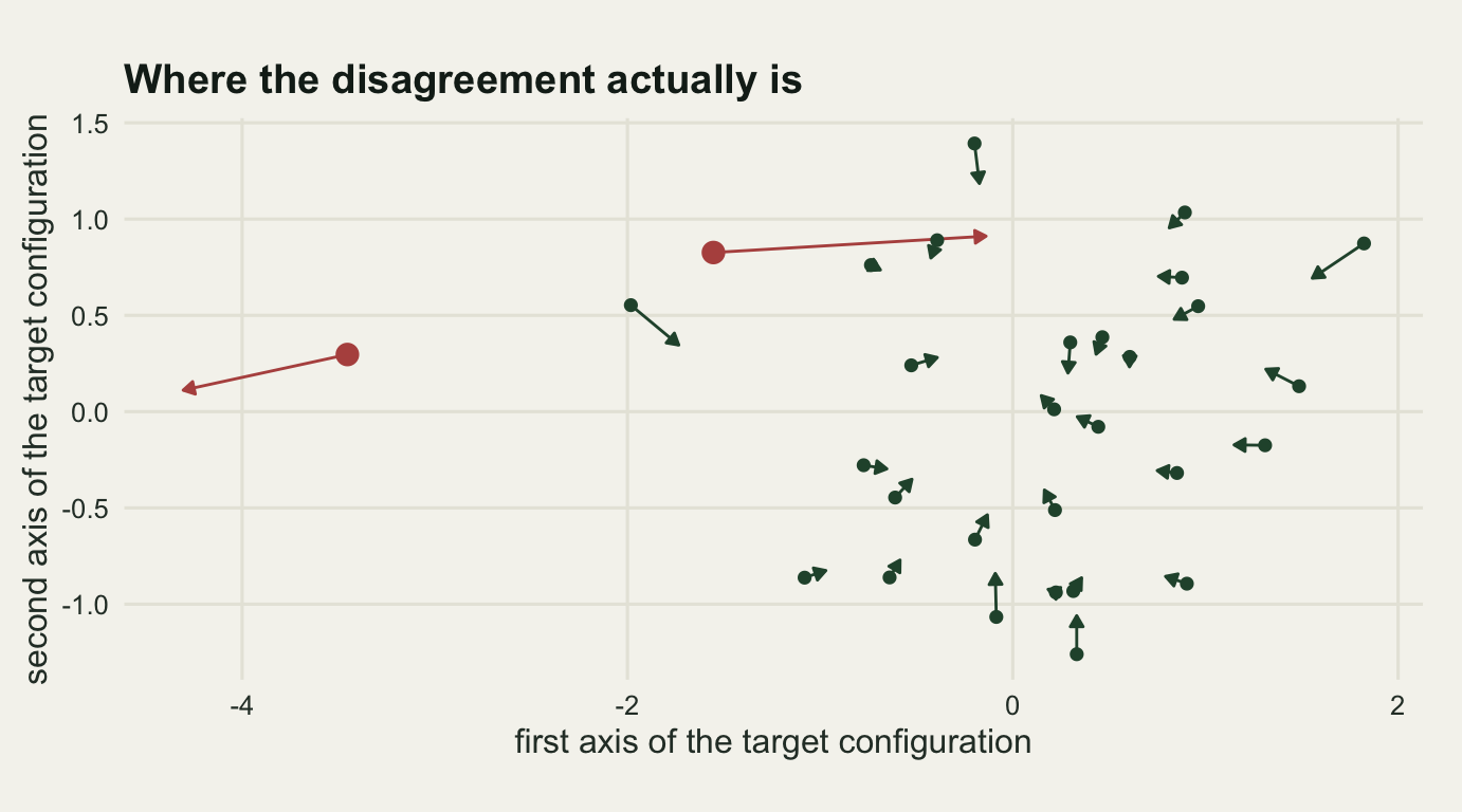
This is the plot vegan::plot.procrustes draws, and it is the reason to draw it rather than report the summary. Two long arrows and twenty-eight stubs is a completely different finding from thirty medium arrows, and \(m^2\) cannot distinguish them.
Two taxonomic groups, one set of sites
Back to the plants and the beetles. Both groups respond to the same underlying gradient, the beetles also respond to a second driver the plants ignore, and both have lognormal overdispersion on top of the Poisson counts. Ordinate each group on its own Bray-Curtis matrix and ask how much the two configurations agree.
sim_group <- function(grad, n_sp, seed, od) {
  set.seed(seed)
  n_s <- length(grad)
  opt <- runif(n_sp, -1, 11)
  tol <- runif(n_sp, 1, 3.5)
  amp <- runif(n_sp, 8, 50)
  mu <- outer(grad, seq_len(n_sp),
              function(g, j) amp[j] * exp(-((g - opt[j])^2) / (2 * tol[j]^2)))
  mu <- mu * exp(matrix(rnorm(length(mu), 0, od), nrow = n_s))
  m <- matrix(rpois(length(mu), mu), nrow = n_s)
  m[, colSums(m) > 0, drop = FALSE]
}

set.seed(6060)
n_plot <- 30
moisture <- sort(runif(n_plot, 0, 10))
second_driver <- rnorm(n_plot)
driver_weight <- 1.6
overdisp <- 0.9

plants <- sim_group(moisture, 35, 101, overdisp)
beetles <- sim_group(moisture + driver_weight * second_driver, 30, 202,
                     overdisp)
pco_pl <- cmdscale(as.dist(bray_hand(plants)), k = 2)
pco_be <- cmdscale(as.dist(bray_hand(beetles)), k = 2)

tax <- protest_hand(pco_pl, pco_be, nperm = 4999, seed = 20260740)
print(round(c(plots = n_plot, plant_species = ncol(plants),
              beetle_species = ncol(beetles),
              second_driver_weight = driver_weight,
              log_overdispersion = overdisp), 4))
plots plant_species beetle_species
30.0 35.0 30.0
second_driver_weight log_overdispersion
1.6 0.9 print(signif(c(procrustes_r = tax$r, m2 = tax$m2, p_value = tax$p,
null_q95 = unname(quantile(tax$perm, 0.95)),
null_mean = mean(tax$perm),
axis1_correlation = cor(pco_pl[, 1], pco_be[, 1])), 5)) procrustes_r m2 p_value null_q95
0.69331 0.51932 0.00020 0.34515
null_mean axis1_correlation
0.20219 0.82318 The Procrustes correlation between the plant configuration and the beetle configuration is 0.6933, with \(m^2\) of 0.5193 and a p-value of 0.0002. The ninety-fifth percentile of the permutation null is 0.3452, so the observed value clears the bar by a wide margin.
Here is where the number needs care. A correlation of 0.69 is a strong result and also a weak one, depending on which question is being asked. As a test against no relationship it is decisive: the null distribution tops out at 0.646 across 4999 permutations and the observed value sits above that, so no permutation reproduced it. As a statement about how much of the beetle configuration the plant configuration accounts for, it leaves 51.9 per cent of the dispersion unmatched. The two groups are ordering the sites along broadly the same gradient and disagreeing about a great deal of the detail. In this simulation we know why: the beetles were given a second driver with weight 1.6 that the plants never saw.
Reporting the correlation without the null distribution beside it is the mistake to avoid, because the null moves.
How much agreement counts as agreement
The permutation null for a Procrustes correlation depends on the number of sites and almost nothing else. With few sites there are few permutations that can be badly wrong, so a random pairing already produces a high correlation and the bar for significance is high; with many sites the bar falls. Measuring it is direct: for each sample size, draw pairs of independent configurations, build the permutation null for each pair, and take the ninety-fifth percentile, averaging over several pairs to smooth the estimate.
crit_r <- function(n_pts, n_pair = 40, nperm = 999, seed) {
  set.seed(seed)
  q <- numeric(n_pair)
  for (k in seq_len(n_pair)) {
    Xi <- unit_conf(matrix(rnorm(n_pts * 2), n_pts, 2))
    Yi <- unit_conf(matrix(rnorm(n_pts * 2), n_pts, 2))
    rp <- numeric(nperm)
    for (b in seq_len(nperm)) {
      rp[b] <- r_two_dim(t(Xi) %*% Yi[sample.int(n_pts), , drop = FALSE])
    }
    q[k] <- quantile(rp, 0.95)
  }
  mean(q)
}

n_grid <- c(10, 20, 30, 40, 80)
crit <- vapply(n_grid, crit_r, numeric(1), seed = 20260741)
crit_tab <- data.frame(n = n_grid, critical_r = crit, critical_m2 = 1 - crit^2)
pow_slope <- unname(coef(lm(log(crit) ~ log(n_grid)))[2])

print(round(crit_tab, 4))
n critical_r critical_m2
1 10 0.6032 0.6361
2 20 0.4298 0.8153
3 30 0.3497 0.8777
4 40 0.3027 0.9084
5 80 0.2141 0.9542print(round(c(fitted_log_log_slope = pow_slope), 4))fitted_log_log_slope
-0.4989 print(round(c(r_needed_at_10 = crit[1], r_needed_at_80 = crit[5],
ratio = crit[1] / crit[5],
sqrt_of_size_ratio = sqrt(80 / 10)), 4)) r_needed_at_10 r_needed_at_80 ratio sqrt_of_size_ratio
0.6032 0.2141 2.8172 2.8284 print(round(c(observed_two_taxa_r = tax$r,
margin_at_10_sites = tax$r - crit[1],
margin_at_80_sites = tax$r - crit[5],
observed_index_r = idx$r), 4))observed_two_taxa_r margin_at_10_sites margin_at_80_sites observed_index_r
0.6933 0.0901 0.4792 0.9693 At ten sites a Procrustes correlation of 0.6032 is what two unrelated configurations reach at the five per cent point, which corresponds to an \(m^2\) of 0.6361. At eighty sites the same threshold is 0.2141. The ratio is 2.817 against 2.828 for the square root of the sample size ratio, and fitting a line through the logarithms gives a slope of -0.4989, near enough the \(n^{-1/2}\) that a correlation-like statistic should follow.
The practical consequence is a table, not a rule of thumb. The plant against beetle correlation of 0.6933 clears the threshold at thirty sites by 0.344. The same value at ten sites would clear it by only 0.09, and at eighty sites by 0.479. A published Procrustes correlation of about 0.7 from a ten-plot pilot is a marginal finding; the identical number from an eighty-plot survey is a comfortable one. Neither is comparable to the other without the sample size attached.
ref_level <- 0.7
obs_df <- data.frame(n = c(n_plot, n_site), r = c(tax$r, idx$r),
                     vj = c(2.0, 0.4),
                     lab = c("plants vs beetles", "Bray-Curtis vs Jaccard"))

ggplot(crit_tab, aes(n, critical_r)) +
  geom_hline(yintercept = ref_level, colour = te_pal$gold, linetype = "22",
             linewidth = 0.8) +
  geom_line(colour = te_pal$forest, linewidth = 0.8) +
  geom_point(colour = te_pal$forest, size = 2.6) +
  geom_point(data = obs_df, aes(n, r), colour = te_pal$clay, shape = 17,
             size = 3.2) +
  geom_text(data = obs_df, aes(n, r, label = lab, vjust = vj),
            colour = te_pal$clay, hjust = -0.13, size = 3.1) +
  scale_x_log10(breaks = n_grid, limits = c(9, 260)) +
  scale_y_log10(breaks = c(0.2, 0.3, 0.5, 0.7, 1.0)) +
  labs(x = "number of sites",
       y = "Procrustes correlation (log scale)",
       title = "The bar for significance falls with sample size") +
  theme_te() +
  theme(plot.margin = margin(8, 16, 4, 8))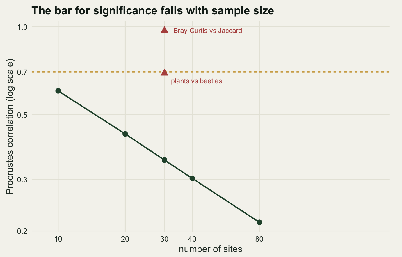
The gold line is a correlation of 0.7. It sits above the threshold curve at every sample size measured, so a result of that size is significant throughout the range, but the gap between them grows from 0.097 at ten sites to 0.486 at eighty. The statistic does not change; what it gets compared against does.
What to take away
Two ordinations of the same sites cannot be compared coordinate by coordinate, and the measurements above put a size on how badly that goes. Across 18 NMDS runs that all reached the same stress on the same dissimilarity matrix, the axis correlations against a reference run ranged from -0.947 to 1 while the Procrustes \(m^2\) never exceeded 0.00593. The axis correlation was measuring the random number generator.
The machinery is small enough to write out: centre both configurations, decompose one crossproduct, and the rotation, the reflection, the scale and the residual all fall out. It recovered a known sixty degree rotation to 7.11e-15 degrees, reproduced a known scale change with an error of 1.11e-16, and matches vegan to 1.42e-14 on the residual sum of squares.
Two results deserve to travel further than the rest. The summary statistic hides where the disagreement lives: two of 30 sites carried 80.4 per cent of the residual sum of squares in the constructed case, and dropping them moved \(m^2\) from 0.0693 to 0.00606, so draw the arrows. And the significance threshold moves with sample size, from 0.603 at ten sites to 0.214 at eighty on a slope of -0.499, so a Procrustes correlation reported without its sample size is not interpretable.
The honest limit is the spatial one, and it is the measurement here I would most want a reader to keep. On configurations independent by construction but smooth over the same site coordinates, the test rejected at 21.3 per cent against a nominal five, an inflation of 4.26. Field surveys are laid out in space and community data is spatially structured almost by definition, so the default permutation scheme tests a null that a real dataset does not satisfy. Procrustes removes the arbitrary part of an ordination cleanly and reports what is left honestly; the p-value beside it is only as good as the exchangeability assumption underneath, and on spatial data that assumption is usually false.
References
Schonemann PH 1966 Psychometrika 31(1):1-10 (10.1007/BF02289451)
Gower JC 1975 Psychometrika 40(1):33-51 (10.1007/BF02291478)
Jackson DA 1995 Ecoscience 2(3):297-303 (10.1080/11956860.1995.11682297)
Peres-Neto PR, Jackson DA 2001 Oecologia 129(2):169-178 (10.1007/s004420100720)
Dray S, Chessel D, Thioulouse J 2003 Ecoscience 10(1):110-119 (10.1080/11956860.2003.11682757)
Lisboa FJG, Peres-Neto PR, Chaer GM, Jesus EC, Mitchell RJ, Chapman SJ, Berbara RLL 2014 PLoS ONE 9(6):e101238 (10.1371/journal.pone.0101238)
Gower JC, Dijksterhuis GB 2004 Procrustes Problems (ISBN 978-0-19-851058-1)
Legendre P, Legendre L 2012 Numerical Ecology, third English edition (ISBN 978-0-444-53868-0)