library(vegan)
library(ggplot2)
te_canvas <- theme(plot.background  = element_rect(fill = "#f5f4ee", colour = NA),
                   panel.background = element_rect(fill = "#f5f4ee", colour = NA))

set.seed(33)

n_sites <- 50
x <- runif(n_sites)
y <- runif(n_sites)

# moisture: west-east gradient (spatial), mild north-south, plus noise
moisture <- 60 + 25 * x + 6 * y + rnorm(n_sites, 0, 6)

# a second driver, not spatially structured and not measured.
# some species track it, so moisture explains only part of the pattern.
z <- rnorm(n_sites, 0, 1)

n_sp   <- 18
opt    <- seq(52, 98, length.out = n_sp)   # moisture optima
width  <- 10
peak   <- 18
z_load <- c(rep(0, 9), runif(9, 0.5, 1.1)) # last nine species respond to z

log_lambda <- outer(moisture, opt,
                    function(m, o) log(peak) - ((m - o)^2) / (2 * width^2)) +
  outer(z, z_load)
comm <- matrix(rpois(n_sites * n_sp, exp(log_lambda)), nrow = n_sites)
colnames(comm) <- paste0("sp", seq_len(n_sp))Mantel tests in R: correlating distance matrices
R
multivariate
spatial statistics
ecology tutorial
Simple and partial Mantel tests with vegan, what they really test, and why a spatially structured environment can make geography look important when it is not.
Updated 27 September 2026: a new section, Choosing the variables, then testing them, measures how often a Mantel test of the subset that bioenv picks rejects a true null, and what the permutation test that reruns the whole search gives instead.
Updated 25 September 2026: a new section, The Mantel correlogram: similarity by distance class, measures on a community with a known spatial range where the significant distance classes stop, and why they stop short of that range.
A Mantel test asks whether two distance matrices covary. In community ecology the usual version is: do sites that differ a lot in their environment also differ a lot in species composition? A partial Mantel adds a third matrix, so you can ask the same question while holding geographic distance constant. The mechanics are a couple of lines in vegan. The interpretation is where most of the trouble lives, so the last section is about what the test really answers and where it tends to mislead.
A landscape where environment and space are tangled
The example uses 50 sites on a unit square. Soil moisture rises from west to east, so moisture carries a spatial pattern of its own. Eighteen species have Gaussian responses to moisture, and a second driver that we never measure also shapes part of the community. That second driver matters: a single measured gradient never explains everything in real data, and leaving some composition unexplained by moisture keeps the example honest.
The moisture gradient is easy to see when you put the sites back on the map.
map_df <- data.frame(x = x, y = y, moisture = moisture)

ggplot(map_df, aes(x, y, fill = moisture)) +
  geom_point(shape = 21, size = 5, colour = "#2c3a31", stroke = 0.5) +
  scale_fill_gradient(low = "#c9b458", high = "#1d5b4e", name = "Soil\nmoisture") +
  coord_equal() +
  labs(x = "Easting (unit square)", y = "Northing (unit square)") +
  theme_minimal(base_size = 13) + te_canvas +
  theme(panel.grid.minor = element_blank(),
        text = element_text(colour = "#2c3a31"))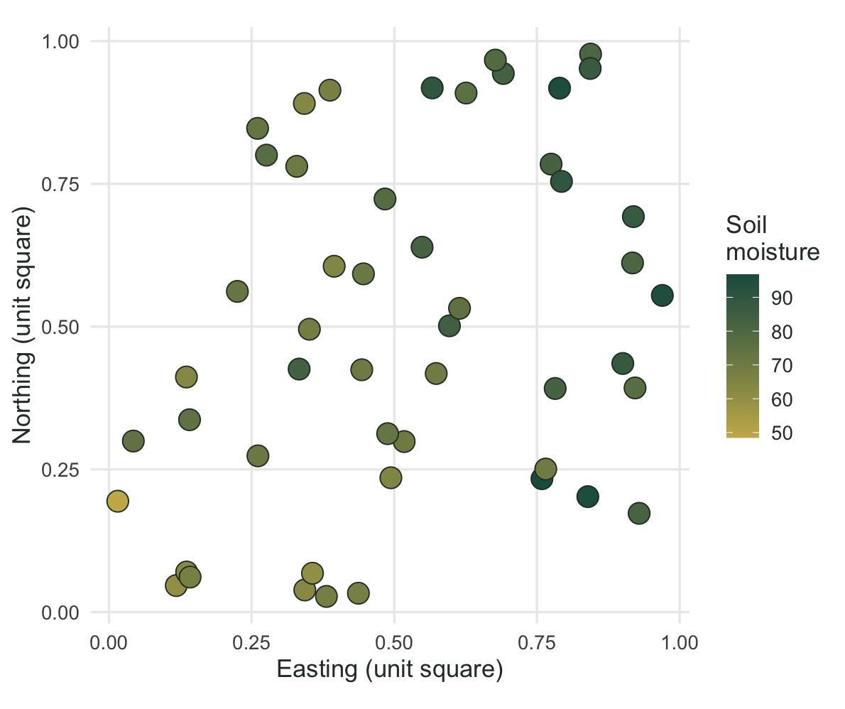
Three distance matrices
A Mantel test never sees the site values directly. It works on distances: one matrix per data source, each holding the pairwise distance between every pair of sites. Here we need three.
comm_d <- vegdist(comm, method = "bray")   # community dissimilarity
env_d  <- dist(scale(moisture))            # environmental distance
geo_d  <- dist(cbind(x, y))                # geographic distance
Community dissimilarity is Bray-Curtis on the abundances. Environmental distance is the absolute difference in scaled moisture. Geographic distance is the straight-line distance on the map. Every Mantel test below is a correlation between two of these three, computed over the lower triangle of the matrices.
The simple Mantel test
Start with the question people usually ask: is community dissimilarity related to environmental distance?
set.seed(33)
mantel(comm_d, env_d, method = "pearson", permutations = 999)
Mantel statistic based on Pearson's product-moment correlation

Call:
mantel(xdis = comm_d, ydis = env_d, method = "pearson", permutations = 999)

Mantel statistic r: 0.7579
      Significance: 0.001

Upper quantiles of permutations (null model):
  90%   95% 97.5%   99%
0.085 0.112 0.138 0.162
Permutation: free
Number of permutations: 999
Sites that differ in moisture differ in composition, which is what the data were built to show. Now run the same test against geographic distance.
set.seed(33)
mantel(comm_d, geo_d, method = "pearson", permutations = 999)
Mantel statistic based on Pearson's product-moment correlation

Call:
mantel(xdis = comm_d, ydis = geo_d, method = "pearson", permutations = 999)

Mantel statistic r: 0.324
      Significance: 0.001

Upper quantiles of permutations (null model):
   90%    95%  97.5%    99%
0.0610 0.0883 0.1074 0.1234
Permutation: free
Number of permutations: 999
This one is positive too, and again significant. Read on its own, that result invites a story about dispersal limitation or spatial structure in the community. Before accepting it, check whether the environment is itself spatial.
set.seed(33)
mantel(env_d, geo_d, method = "pearson", permutations = 999)
Mantel statistic based on Pearson's product-moment correlation

Call:
mantel(xdis = env_d, ydis = geo_d, method = "pearson", permutations = 999)

Mantel statistic r: 0.4036
      Significance: 0.001

Upper quantiles of permutations (null model):
   90%    95%  97.5%    99%
0.0626 0.0802 0.0962 0.1114
Permutation: free
Number of permutations: 999
Environmental distance and geographic distance are positively correlated as well. Moisture is patterned in space, so two sites that are far apart tend to differ in moisture, and therefore in composition. The community-geography correlation might be nothing more than the spatial footprint of moisture. The scatterplots make the difference in signal plain.
set.seed(33)
r_env <- mantel(comm_d, env_d, permutations = 999)$statistic
set.seed(33)
r_geo <- mantel(comm_d, geo_d, permutations = 999)$statistic

dd_long <- data.frame(
  comm = rep(as.vector(comm_d), 2),
  dist = c(as.vector(env_d), as.vector(geo_d)),
  type = rep(c(
    sprintf("community vs environment   (Mantel r = %.2f)", r_env),
    sprintf("community vs geography   (Mantel r = %.2f)", r_geo)
  ), each = length(comm_d))
)

ggplot(dd_long, aes(dist, comm)) +
  geom_point(alpha = 0.22, colour = "#275139", size = 1.2) +
  geom_smooth(method = "lm", formula = y ~ x, se = FALSE, colour = "#b5534e", linewidth = 1) +
  facet_wrap(~ type, scales = "free_x") +
  labs(x = "Pairwise distance between sites",
       y = "Community dissimilarity (Bray-Curtis)") +
  theme_minimal(base_size = 12) + te_canvas +
  theme(panel.grid.minor = element_blank(),
        strip.text = element_text(face = "bold", size = 10),
        text = element_text(colour = "#2c3a31"))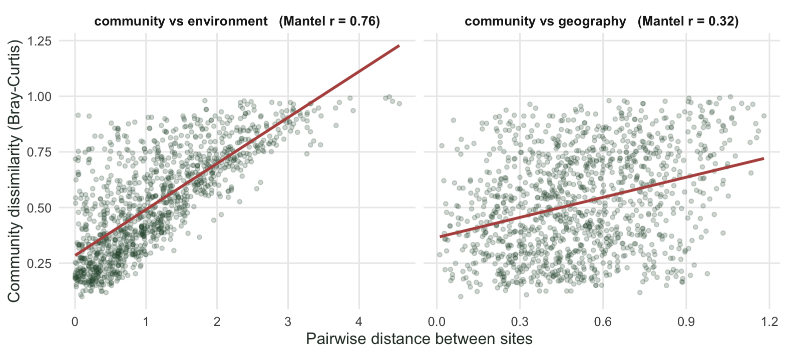
The partial Mantel test
A partial Mantel correlates two matrices while holding a third constant, in the same spirit as partial correlation on ordinary variables. mantel.partial() takes the three matrices in order: the two being correlated, then the one being controlled for.
set.seed(33)
pm_env <- mantel.partial(comm_d, env_d, geo_d, method = "pearson", permutations = 999)
pm_env
Partial Mantel statistic based on Pearson's product-moment correlation

Call:
mantel.partial(xdis = comm_d, ydis = env_d, zdis = geo_d, method = "pearson",      permutations = 999)

Mantel statistic r: 0.7245
      Significance: 0.001

Upper quantiles of permutations (null model):
   90%    95%  97.5%    99%
0.0862 0.1093 0.1368 0.1592
Permutation: free
Number of permutations: 999
Controlling for geography, the community-environment correlation moves from 0.76 to 0.72. Now reverse the roles and control for the environment instead.
set.seed(33)
mantel.partial(comm_d, geo_d, env_d, method = "pearson", permutations = 999)
Partial Mantel statistic based on Pearson's product-moment correlation

Call:
mantel.partial(xdis = comm_d, ydis = geo_d, zdis = env_d, method = "pearson",      permutations = 999)

Mantel statistic r: 0.03033
      Significance: 0.27

Upper quantiles of permutations (null model):
   90%    95%  97.5%    99%
0.0702 0.0877 0.1019 0.1228
Permutation: free
Number of permutations: 999
The apparent role of distance was borrowed from moisture. That matches the simulation: nothing connects composition to raw coordinates except through moisture, and once moisture is held constant, position on the map carries almost no information about which species are present.
The Mantel correlogram: similarity by distance class
A Mantel correlogram is a series of Mantel tests, one per distance class, an idea from the mid-1980s work of Sokal and Oden (Oden & Sokal 1986). For each class you build a model matrix that marks the pairs of sites whose geographic distance falls in that class, and correlate it with the community dissimilarity matrix. vegan::mantel.correlog() flips the sign so that a positive Mantel r means pairs in that class are more alike than the average pair, and a negative r means they are less alike. Each class gets a permutation test, one-tailed in the direction of its observed r, and by default the p-values get a progressive correction: the test for class k is Holm-corrected together with the k - 1 classes before it, so the largest possible penalty grows as you read outwards from the shortest distances. The number of classes comes from Sturges’ rule unless you set n.class or break.pts, and with the default cutoff = TRUE only the first half of the classes is tested, plus any later class in which every site still has a partner.
The tempting reading is that the distance where significant positive values stop is the scale of the spatial pattern. To check that reading we need a community whose range we know. The moisture gradient above is a straight west-east trend, which has no range at all, so the next block builds a separate one: 100 sites on the unit square, a latent environmental field with a spherical covariance whose correlation is exactly zero beyond a distance of 0.3, and 20 species with Gaussian responses to that field. The field in the Moran’s I post has an exponential covariance, which fades without ever reaching zero; the spherical model gives the range a hard edge to measure against.
# a community with a known spatial range: base R, own seed
sph_cor  <- function(h, a) ifelse(h < a, 1 - 1.5 * h / a + 0.5 * (h / a)^3, 0)
range_cg <- 0.3                               # field correlation is zero beyond this
n_cg     <- 100
opt_cg   <- seq(-2.2, 2.2, length.out = 20)   # species optima along the field

sim_patchy <- function() {
  xy <- cbind(runif(n_cg), runif(n_cg))
  h  <- as.matrix(dist(xy))
  field  <- drop(crossprod(chol(sph_cor(h, range_cg) + diag(1e-8, n_cg)), rnorm(n_cg)))
  lambda <- exp(log(15) - outer(field, opt_cg, "-")^2 / (2 * 0.7^2))
  list(xy = xy, h = h, comm = matrix(rpois(length(lambda), lambda), n_cg))
}

set.seed(1986)
patchy   <- sim_patchy()
patchy_d <- vegdist(patchy$comm, method = "bray")

set.seed(1986)
cg_vegan <- mantel.correlog(patchy_d, XY = patchy$xy, nperm = 999)
round(cg_vegan$mantel.res[1:9, ], 3)
class.index n.dist Mantel.cor Pr(Mantel) Pr(corrected)
D.cl.1 0.053 318 0.088 0.001 0.001
D.cl.2 0.141 648 0.075 0.001 0.002
D.cl.3 0.229 936 0.002 0.449 0.449
D.cl.4 0.317 1132 -0.045 0.010 0.020
D.cl.5 0.404 1176 -0.063 0.001 0.005
D.cl.6 0.492 1268 -0.045 0.002 0.006
D.cl.7 0.580 1228 -0.014 0.179 0.358
D.cl.8 0.668 1134 0.009 0.267 0.537
D.cl.9 0.756 912 NA NA NAThe permutation p-values in that table move a little from one run to the next, and between vegan versions, so the figure and the numbers quoted below come from a base-R version of the same calculation with its own seed. It applies the same class breaks, cutoff rule and progressive Holm correction, and the block ends by checking that its Mantel r values match vegan’s to 12 decimal places.
low_cg <- lower.tri(diag(n_cg))
pair_i <- row(diag(n_cg))[low_cg]
pair_j <- col(diag(n_cg))[low_cg]

# one column of pairwise dissimilarities per permutation of the site labels
perm_dissim <- function(dmat, nperm) {
  perms <- replicate(nperm, sample.int(n_cg))
  matrix(dmat[(perms[pair_j, ] - 1) * n_cg + perms[pair_i, ]], ncol = nperm)
}

mantel_correlog_base <- function(dv, hv, dperm, n_class) {
  brk  <- seq(min(hv), max(hv), length.out = n_class + 1)
  cls  <- factor(pmax(findInterval(hv, brk, left.open = TRUE), 1), levels = seq_len(n_class))
  n_in <- tabulate(cls, n_class)
  n_pr <- length(dv)
  # Pearson r between dissimilarity and the 0/1 class matrix, sign flipped as in vegan
  r_cls  <- -(tapply(dv, cls, mean) - mean(dv)) *
    sqrt(n_in * n_pr / (n_pr - n_in)) / (sd(dv) * sqrt(n_pr - 1))
  s_obs  <- rowsum(dv, cls, reorder = TRUE)[, 1]
  s_perm <- rowsum(dperm, cls, reorder = TRUE)
  covers <- sapply(seq_len(n_class), function(k)
    length(unique(c(pair_i[cls == k], pair_j[cls == k]))) == n_cg)
  tested <- n_in > 0 & (seq_len(n_class) <= n_class %/% 2 | covers)
  p_raw  <- ifelse(r_cls > 0, rowSums(s_perm <= s_obs), rowSums(s_perm >= s_obs))
  p_raw  <- (p_raw + 1) / (ncol(dperm) + 1)
  p_raw[!tested] <- NA
  p_prog <- sapply(seq_len(n_class), function(k)
    if (tested[k]) p.adjust(p_raw[1:k], "holm")[k] else NA)
  data.frame(lo = head(brk, -1), hi = brk[-1], mid = (head(brk, -1) + brk[-1]) / 2,
             r = unname(r_cls), p_raw = unname(p_raw), p_prog = p_prog)
}

patchy_m <- as.matrix(patchy_d)
set.seed(2012)
cg_base <- mantel_correlog_base(patchy_m[low_cg], patchy$h[low_cg],
                                perm_dissim(patchy_m, 999), n_class = 14)
stopifnot(max(abs(cg_base$r - cg_vegan$mantel.res[, "Mantel.cor"]), na.rm = TRUE) < 1e-12)
cg_sig <- !is.na(cg_base$p_prog) & cg_base$p_prog <= 0.05
cg_plot <- cg_base[!is.na(cg_base$p_prog), ] # the classes vegan tests
cg_plot$verdict <- factor(ifelse(cg_plot$p_prog > 0.05, "not significant",
ifelse(cg_plot$r > 0, "more alike, p <= 0.05", "less alike, p <= 0.05")),
levels = c("more alike, p <= 0.05", "less alike, p <= 0.05", "not significant"))
ggplot(cg_plot, aes(mid, r)) +
geom_hline(yintercept = 0, colour = "#dad9ca", linewidth = 0.7) +
geom_vline(xintercept = range_cg, linetype = "22", colour = "#16241d") +
annotate("text", x = range_cg + 0.015, y = max(cg_plot$r) * 0.98, hjust = 0,
label = "true range of the field", colour = "#16241d", size = 3.6) +
geom_line(colour = "#2c3a31", linewidth = 0.5) +
geom_point(aes(fill = verdict), shape = 21, size = 3.4, colour = "#2c3a31", stroke = 0.5) +
scale_fill_manual(values = c("more alike, p <= 0.05" = "#275139",
"less alike, p <= 0.05" = "#b5534e",
"not significant" = "#c9b458"), drop = FALSE, name = NULL) +
scale_x_continuous(breaks = seq(0, 0.7, by = 0.1)) +
labs(x = "Geographic distance (class midpoint)", y = "Mantel r") +
theme_minimal(base_size = 12) + te_canvas +
theme(panel.grid.minor = element_blank(), legend.position = "top",
text = element_text(colour = "#2c3a31"))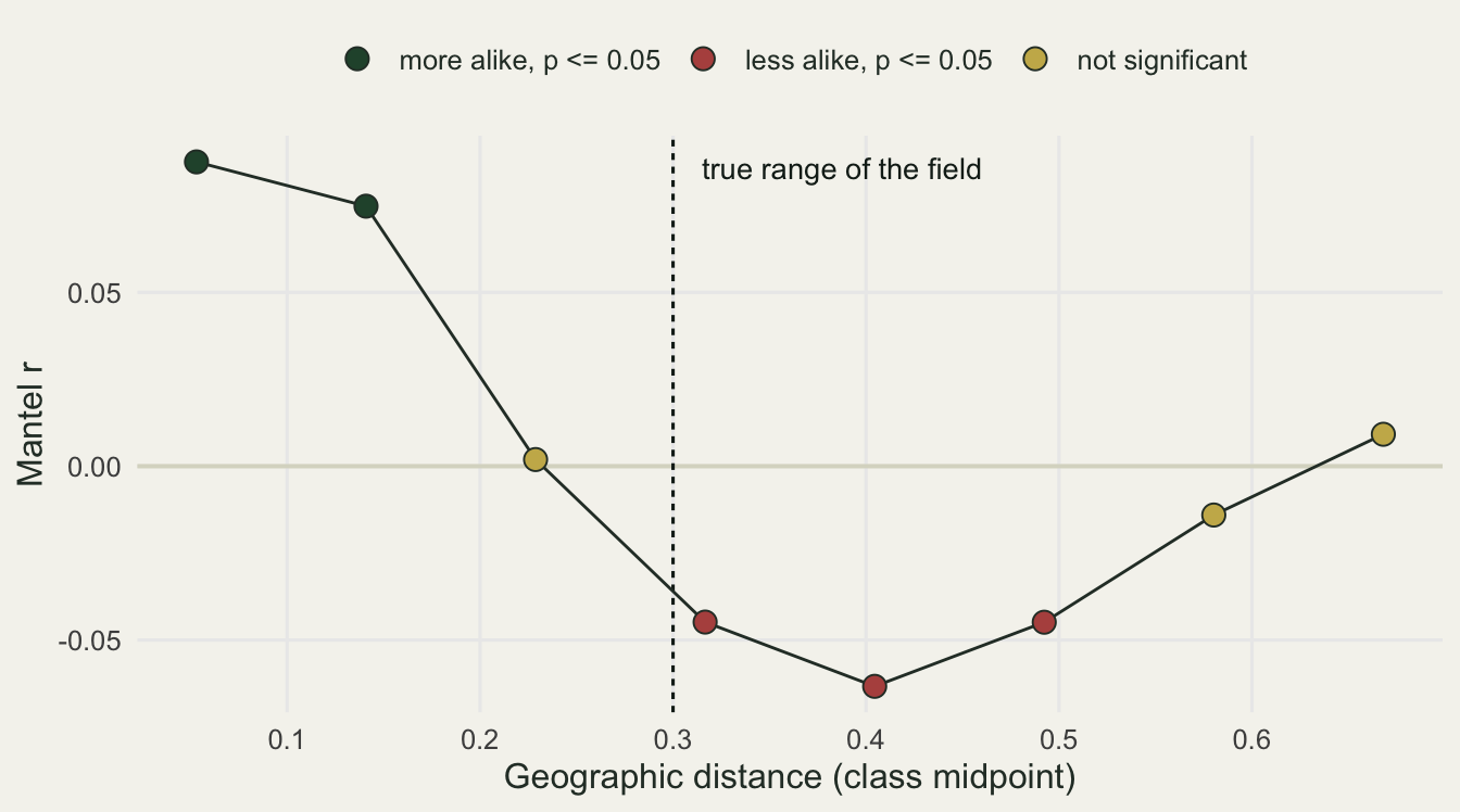
The first two classes, out to a distance of 0.18, are significantly more alike than the average pair (Mantel r of 0.088 and 0.075). The third class, from 0.18 to 0.27, has r = 0.002 and is not significant, although it lies entirely inside the range: two sites at those distances still share a field correlation of 0.01 to 0.19. The next three classes, from 0.27 to 0.54, are significantly less alike than the average pair, and all but the first of them lie wholly beyond the range, where the field carries no correlation at all. So significant positive autocorrelation ends well inside the range, and past the range the correlogram does not return to zero.
The negative stretch is arithmetic, not biology. Beyond the range every pair is, in expectation, as different as two unrelated sites. The average pair, which is what each class is compared with, includes the close and similar pairs, so a class made only of unrelated pairs is less alike than average and the Mantel r comes out negative. With enough pairs in the class, that difference is significant.
The same arithmetic pulls the zero crossing inside the range. A class whose pairs are only weakly linked is still less alike than the average pair, so its expected r is already negative. The next block computes, for this design and without any permutation test, the expected Bray-Curtis dissimilarity at each distance from the field correlation alone, and compares it with the average over all pairs of points in the unit square.
# the expected correlogram, no test involved: own seed, base R
set.seed(1926)
n_zmc <- 20000                                   # simulated pairs of sites
cg_z1 <- rnorm(n_zmc)
cg_z2 <- rnorm(n_zmc)
# counts at a site with field value f, from the same species model as sim_patchy()
cg_counts <- function(f)
  matrix(rpois(n_zmc * length(opt_cg), exp(log(15) - outer(f, opt_cg, "-")^2 / (2 * 0.7^2))), n_zmc)
cg_site1 <- cg_counts(cg_z1)

# mean Bray-Curtis dissimilarity of two sites whose field values have correlation rho
rho_grid <- seq(0, 1, by = 0.02)
bray_rho <- sapply(rho_grid, function(rho) {
  site2 <- cg_counts(rho * cg_z1 + sqrt(1 - rho^2) * cg_z2)
  mean(rowSums(abs(cg_site1 - site2)) / rowSums(cg_site1 + site2), na.rm = TRUE)
})

# the average pair: distances between random pairs of points in the unit square
h_mc   <- sqrt((runif(n_zmc * 25) - runif(n_zmc * 25))^2 + (runif(n_zmc * 25) - runif(n_zmc * 25))^2)
bray_h <- approx(rho_grid, bray_rho, sph_cor(h_mc, range_cg))$y

# first distance at which the expected dissimilarity reaches that of the average pair
h_grid <- seq(0, range_cg, by = 0.001)
h_zero <- h_grid[which.max(approx(rho_grid, bray_rho, sph_cor(h_grid, range_cg))$y >= mean(bray_h))]
round(c(unrelated_pair = bray_rho[1], average_pair = mean(bray_h),
        zero_crossing = h_zero, field_cor_there = sph_cor(h_zero, range_cg)), 3)
unrelated_pair average_pair zero_crossing field_cor_there
0.532 0.523 0.236 0.063 The expected correlogram crosses zero at a distance of 0.24, or 0.79 of the range, where the field correlation has fallen to 0.06. That point falls inside the third class of Figure 3. So even averaged over many fields, and before any test is run, the positive part of the correlogram ends short of 0.3; with a real sample, limited power moves the end point further in.
One community is one draw. The next block repeats the whole thing on 150 fresh communities with the same design and records, for each, where the unbroken run of significant positive classes ends (the upper edge of its last class). It does this at the default 14 classes and at half and double that number; the three class designs share one set of 999 permutations per community.
where_it_stops <- function(cg) {
  sig    <- !is.na(cg$p_prog) & cg$p_prog <= 0.05
  run    <- sum(cumprod(sig & cg$r > 0))      # length of the first run of positive classes
  run_raw <- sum(cumprod(!is.na(cg$p_raw) & cg$p_raw <= 0.05 & cg$r > 0))   # same, uncorrected
  beyond <- cg$lo >= range_cg & !is.na(cg$p_prog)
  c(stop = if (run > 0) cg$hi[run] else 0, run = run,
    stop_raw = if (run_raw > 0) cg$hi[run_raw] else 0,
    neg_beyond = any(sig[beyond] & cg$r[beyond] < 0),
    pos_beyond = any(sig[beyond] & cg$r[beyond] > 0))
}

n_rep_cg <- 150
set.seed(2012)
mc_cg <- do.call(rbind, lapply(seq_len(n_rep_cg), function(i) {
  sim <- sim_patchy()
  dm  <- as.matrix(vegdist(sim$comm, method = "bray"))
  dp  <- perm_dissim(dm, 999)
  do.call(rbind, lapply(c(7, 14, 28), function(k)
    data.frame(n_class = k,
               t(where_it_stops(mantel_correlog_base(dm[low_cg], sim$h[low_cg], dp, k))))))
}))

stop_tab <- do.call(rbind, lapply(split(mc_cg, mc_cg$n_class), function(s)
  data.frame(n_class = s$n_class[1], below = mean(s$stop < range_cg),
             median_stop = median(s$stop), neg_beyond = mean(s$neg_beyond))))
stop_tab$se_below <- sqrt(stop_tab$below * (1 - stop_tab$below) / n_rep_cg)
stop_tab
n_class below median_stop neg_beyond se_below
7 7 0.8333333 0.1918383 0.6200000 0.03042903
14 14 0.9133333 0.1909379 0.6066667 0.02297180
28 28 0.9666667 0.1538220 0.4800000 0.01465656stop_n <- function(k) sum(mc_cg$stop[mc_cg$n_class == k] < range_cg)
neg_n <- function(k) sum(mc_cg$neg_beyond[mc_cg$n_class == k])
pos_n <- function(k) sum(mc_cg$pos_beyond[mc_cg$n_class == k])
raw_n <- function(k) sum(mc_cg$stop_raw[mc_cg$n_class == k] < range_cg)
stop_w <- split(mc_cg$stop, mc_cg$n_class) # one value per community, same order in each class design
earlier <- sum(stop_w[["28"]] < stop_w[["14"]])
later <- sum(stop_w[["28"]] > stop_w[["14"]])
brk7 <- seq(min(patchy$h[low_cg]), max(patchy$h[low_cg]), length.out = 8)
past7 <- with(mc_cg[mc_cg$n_class == 7, ], c(past = sum(stop >= range_cg), via_second = sum(stop >= range_cg & run == 2)))
past7 past via_second
25 21 mc_cg$classes <- factor(paste(mc_cg$n_class, "classes"),
levels = paste(c(7, 14, 28), "classes"))
ggplot(mc_cg, aes(stop, colour = classes)) +
geom_vline(xintercept = range_cg, linetype = "22", colour = "#16241d") +
annotate("text", x = range_cg + 0.008, y = 0.08, hjust = 0,
label = "true range of the field", colour = "#16241d", size = 3.6) +
stat_ecdf(geom = "step", linewidth = 0.9) +
scale_colour_manual(values = c("#c9b458", "#275139", "#b5534e"), name = NULL) +
labs(x = "Distance where significant positive autocorrelation ends",
y = "Share of simulated communities") +
theme_minimal(base_size = 12) + te_canvas +
theme(panel.grid.minor = element_blank(), legend.position = "top",
text = element_text(colour = "#2c3a31"))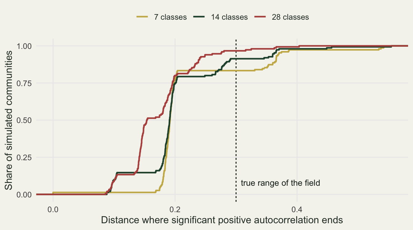
With the default 14 classes, the run of significant positive classes ended short of the true range in 137 of the 150 communities (Monte Carlo standard error of that share 0.023), and the median end point was 0.19, or 0.64 of the range. Finer classes stop earlier: in 79 communities the 28-class run ended before the 14-class run, and in 15 after it; with 28 classes the count rises to 145 and the median end falls to 0.15. A narrow class holds fewer pairs, so its test has less power. The progressive correction is not what moves the end point: judged on the uncorrected p-values, the counts are 137 with 14 classes and 144 with 28, almost the same as with it. With 7 classes the count is 125. That coarse grid has its own trap: the second of seven classes straddles the range (for the community in Figure 3 it would run from 0.18 to 0.36), so when it is significant the run ends past 0.3 by construction, and 21 of the 25 seven-class runs that ended past the range ended there. The negative stretch was common too: with 14 classes, 91 of the 150 communities had at least one class lying wholly beyond the range that was significantly less alike than average. The opposite turned up as well: in 31 of the 150 a class lying wholly beyond the range was significantly more alike than average, although the field links no pairs there.
So read the end of the significant positive run as a distance that usually falls short of the range (it went past 0.3 in only 13 of the 150 communities with 14 classes), not as the range itself. Read a significant negative stretch after it as what a patchy field with a finite range produces on its own, which does not by itself point to regular spacing, and do not take a significant positive class further out as proof of a second scale of pattern. Report the class breaks, the number of classes and the correction alongside the correlogram, because the end point moves with them. This is not a claim that the test is weak: Borcard & Legendre (2012) found the power of the Mantel correlogram close to that of Moran and Geary correlograms on single variables. The point is that the correlogram answers where pairs are more alike than the average pair, and then only where the difference is detectable, and that distance is shorter than the distance at which the process stops linking sites. The simulation has one range, one sampling density and one community model, so the ratios above belong to this design rather than being general constants.
Choosing the variables, then testing them
Every test so far compared matrices that were fixed before anyone looked at the data. A common workflow picks one of them from the data. bioenv() in vegan, named after the BIO-ENV procedure of Clarke & Ainsworth (1993), which the PRIMER software offers inside its BEST routine, scales a set of environmental variables and searches every subset for the one whose Euclidean distances have the highest Spearman correlation with the community dissimilarities. The natural next step is a Mantel test of the winning subset, and that test answers the wrong question: it asks whether this subset, named in advance, matches the community better than chance, when the subset was chosen because it matched best. The Note on the ?bioenv help page points to mantel() for significance and then warns that tests which assume the variables were chosen in advance are biased, and Clarke, Somerfield & Gorley (2008) named the selection bias and gave the repair, a global BEST test that permutes the samples, reruns the entire search on each permutation and compares the observed maximum with those null maxima. It is the repair used in climate window analysis and, with null maps, in optimising a resistance surface. The block below demonstrates both the bias and the repair on the help-page example (lichen pastures at 24 sites, varespec and varechem), not on the simulated landscape above, and then on the same six variables plus the other eight columns of varechem. The search is written out by hand so that thousands of null searches stay cheap, and the chunk stops if it does not reproduce bioenv() on the real data.
data("varespec", "varechem", package = "vegan")
stopifnot(dim(varespec) == c(24, 44), dim(varechem) == c(24, 14), abs(sum(varespec) - 2417.72) < 1e-6)
env6  <- with(varechem, data.frame(logN = log(N), P, K, Ca, pH, Al))   # the ?bioenv example
env14 <- cbind(env6, varechem[, c("Mg", "S", "Fe", "Mn", "Zn", "Mo", "Baresoil", "Humdepth")])
be_d  <- vegdist(wisconsin(varespec), method = "bray")
sol6  <- bioenv(wisconsin(varespec) ~ log(N) + P + K + Ca + pH + Al, varechem)
invisible(capture.output(sol14 <- bioenv(be_d, env14)))      # silences its progress line
n_be <- nrow(varespec); low_be <- lower.tri(diag(n_be))
be_i <- row(diag(n_be))[low_be]; be_j <- col(diag(n_be))[low_be]
unit_c <- function(m) { m <- sweep(as.matrix(m), 2, colMeans(as.matrix(m))); sweep(m, 2, sqrt(colSums(m^2)), "/") }
comm_mat <- matrix(0, n_be, n_be); comm_mat[low_be] <- rank(be_d); comm_mat <- comm_mat + t(comm_mat)
# relabelling the sites permutes the pairs; Pearson on centred ranks = Spearman
perm_comm <- function(nperm) unit_c(replicate(nperm, { s <- sample.int(n_be); comm_mat[cbind(s[be_i], s[be_j])] }))
best_subset_null <- function(env, n_null, n_inner = 999, batch = 100) {
  sc <- scale(env); d2 <- (sc[be_i, , drop = FALSE] - sc[be_j, , drop = FALSE])^2
  subs <- as.matrix(expand.grid(rep(list(0:1), ncol(env))))[-1, , drop = FALSE]
  rk <- unit_c(apply(sqrt(d2 %*% t(subs)), 2, rank))          # every subset, ranked distances
  r_obs <- drop(crossprod(unit_c(rank(be_d)), rk)); win <- which.max(r_obs)
  fixed <- drop(crossprod(perm_comm(n_inner), rk[, win]))     # naive Mantel of the real winner
  nul <- do.call(rbind, lapply(split(seq_len(n_null), ceiling(seq_len(n_null) / batch)), function(ix) {
    rr <- crossprod(perm_comm(length(ix)), rk)                 # null data: rerun the whole search
    pick <- max.col(rr, ties.method = "first"); mx <- apply(rr, 1, max); cols <- unique(pick)
    inner <- crossprod(perm_comm(n_inner), rk[, cols, drop = FALSE])   # naive Mantel, fresh permutations
    hits <- colSums(inner[, match(pick, cols), drop = FALSE] >= rep(mx, each = n_inner))
    cbind(batch = ix[1], max_rho = mx, reject = (1 + hits) / (n_inner + 1) <= 0.05) }))
  by_batch <- tapply(nul[, "reject"], nul[, "batch"], mean)   # batches give the Monte Carlo error
  list(n_sub = nrow(subs), vars = colnames(env)[subs[win, ] == 1], rho = r_obs[win], fixed_rho = fixed,
       n_close = sum(r_obs >= r_obs[win] - 0.02), naive_p = (1 + sum(fixed >= r_obs[win])) / (n_inner + 1),
       n_beat = sum(nul[, "max_rho"] >= r_obs[win]), global_p = (1 + sum(nul[, "max_rho"] >= r_obs[win])) / (n_null + 1),
       type1 = mean(nul[, "reject"]), type1_se = sd(by_batch) / sqrt(length(by_batch)), n_null = n_null,
       max_rho = nul[, "max_rho"])
}
set.seed(2748); bst6  <- best_subset_null(env6, 9999)
bst14 <- best_subset_null(env14, 2000)
be_ok <- function(b, s) with(s$models[[s$whichbest]], abs(b$rho - est) < 1e-12 && identical(b$vars, s$names[best]))
stopifnot(be_ok(bst6, sol6), be_ok(bst14, sol14))            # the hand-coded search is bioenv()
mc_se <- function(p, n) sqrt(p * (1 - p) / n)
round(t(sapply(list(six = bst6, fourteen = bst14), function(b) c(subsets = b$n_sub, rho = b$rho,
  naive_p = b$naive_p, global_p = b$global_p, null_sets = b$n_null, naive_type1 = b$type1, se_type1 = b$type1_se))), 4)
subsets rho naive_p global_p null_sets naive_type1 se_type1
six 63 0.4005 0.001 0.0086 9999 0.2993 0.0047
fourteen 16383 0.5031 0.001 0.0035 2000 0.7310 0.0118null_df <- do.call(rbind, Map(function(b, lab) data.frame(rho = c(b$fixed_rho, b$max_rho), set = lab, obs = b$rho,
what = rep(c("winning subset, held fixed", "best subset of each null search"), c(length(b$fixed_rho), b$n_null))),
list(bst6, bst14), c("6 candidates, 63 subsets", "14 candidates, 16383 subsets")))
null_df$set <- factor(null_df$set, levels = unique(null_df$set))
ggplot(null_df, aes(rho, fill = what)) +
geom_histogram(aes(y = after_stat(density)), binwidth = 0.02, boundary = 0, position = "identity", alpha = 0.7) +
geom_vline(data = unique(null_df[c("set", "obs")]), aes(xintercept = obs), colour = "#b5534e", linewidth = 0.9) +
facet_wrap(~ set) + scale_x_continuous(breaks = seq(-0.2, 0.6, by = 0.2)) +
scale_fill_manual(values = c("winning subset, held fixed" = "#c9b458",
"best subset of each null search" = "#275139"), name = NULL) +
labs(x = "Spearman Mantel rho", y = "Density") +
theme_minimal(base_size = 12) + te_canvas +
theme(panel.grid.minor = element_blank(), legend.position = "top", panel.spacing = unit(1.5, "lines"),
strip.text = element_text(face = "bold", size = 10), text = element_text(colour = "#2c3a31"))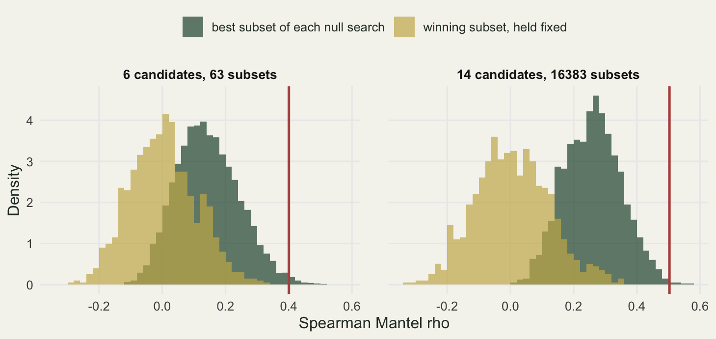
With the six help-page variables the search tries 63 subsets and returns P, Ca, Al with rho = 0.400, and the naive Mantel test of that subset gives p = 0.001, the smallest value its 999 permutations allow. On data where the null is true by construction (the sites of the community relabelled at random, so no subset carries any information), the same two steps rejected at the 5 per cent level in 0.299 of 9999 null data sets (Monte Carlo standard error 0.005, from the spread between batches of 100 null data sets), 6.0 times the nominal rate; with all 14 candidates and 16383 subsets it was 0.731 of 2000 (standard error 0.012). Sixty-three independent tests would reject at least once with probability 1 - 0.95^63 = 0.96; the subsets share variables, so their correlations rise and fall together and the search runs far fewer effective tests than it counts, the point climate window analysis makes about overlapping windows. The figure shows the gap the naive test ignores: the 95th percentile of rho for P, Ca, Al held fixed is 0.18, while the best of the 63 subsets reaches 0.32 at its 95th percentile under the null, and the best of 16383 reaches 0.41.
Both real results survive the correct test. For P, Ca, Al, 85 of the 9999 null searches found a subset at least as good, a global p of 0.0086 (Monte Carlo standard error 0.0009) rather than the naive 0.001; the 14-variable winner, P, Al, Mg, Fe, Mn, Mo, Humdepth with rho = 0.503, was matched or beaten by 6 of 2000, p = 0.0035 (standard error 0.0013). The global test says that the best match beats what the same search finds in noise, not which variables do the work: with 14 candidates, 69 subsets, the winner included, have a rho within 0.02 of the winner’s, an arbitrary small margin (2 with six). The rates above belong to these 24 sites and the correlations among these candidates, and another data set will give other rates. Report the number of candidate variables, the global p and its number of permutations, and not the Mantel p of the winner.
What the Mantel test actually tests
This is the part to read twice. The partial Mantel result above is clean because the data were built for it, but the same machinery gets used on real data to answer a question it was not designed for, and the literature has been clear about the problem for over a decade.
The null hypothesis of a Mantel test is not the null hypothesis of an ordinary correlation. A Pearson correlation between two variables asks whether the variables themselves are associated. A Mantel test asks whether the distances derived from them are associated. Those are different questions, the test statistics behave differently, and rejecting one null does not imply rejecting the other (Legendre, Fortin & Borcard 2015).
For the specific and very common goal of testing a species-environment relationship while accounting for space, that gap has real consequences. Simulation studies show that when both matrices carry spatial autocorrelation, the simple and partial Mantel tests can have inflated type I error and low power, and the partial test does not fix the bias the way people assume it does (Guillot & Rousset 2013; Legendre, Fortin & Borcard 2015). The recommended alternative is to bring space into the model directly, as spatial eigenfunctions (distance-based Moran eigenvector maps), and then partition the variation with redundancy analysis. The variation partitioning post walks through that workflow, and the dbRDA post covers the constrained ordination it rests on.
So when is a Mantel test the right tool? When distances are genuinely the objects of study rather than a stand-in for variables. Isolation by distance in population genetics fits, because the hypothesis is literally about genetic distance against geographic distance. Comparing two independently measured dissimilarity matrices fits, for example asking whether morphological distance tracks genetic distance. And describing the scale of community turnover fits: a Mantel correlogram, as in the correlogram section above, shows how community similarity decays across distance classes, which is more informative than a single coefficient. Reach for the Mantel test when the question is about distances. When the question is about variables and you want to control for space, partition variation instead.
References
Borcard D, Legendre P 2012 Ecology 93(6):1473-1481 (10.1890/11-1737.1)
Clarke KR, Ainsworth M 1993 Marine Ecology Progress Series 92:205-219 (10.3354/meps092205)
Clarke KR, Somerfield PJ, Gorley RN 2008 Journal of Experimental Marine Biology and Ecology 366(1-2):56-69 (10.1016/j.jembe.2008.07.009)
Guillot G, Rousset F 2013 Methods in Ecology and Evolution 4(4):336-344 (10.1111/2041-210x.12018)
Legendre P, Fortin M-J, Borcard D 2015 Methods in Ecology and Evolution 6(11):1239-1247 (10.1111/2041-210X.12425)
Mantel N 1967 Cancer Research 27(2):209-220
Oden NL, Sokal RR 1986 Systematic Zoology 35(4):608-617 (10.2307/2413120)
Smouse PE, Long JC, Sokal RR 1986 Systematic Zoology 35(4):627-632 (10.2307/2413122)