---
title: "Two-species point patterns: testing for interaction"
description: "Toroidal shift and random labelling ask different questions of two mapped species, and on shared habitat one of them fires over tenfold too often. Tested in R."
date: "2026-08-06 15:00"
categories: [R, point patterns, spatial ecology, null models, ecology tutorial]
image: thumbnail.png
image-alt: "Two panels side by side on one shared scale, with distance r from about 0.02 to 0.16 across and a vertical scale from 0.00 to 0.15. Each panel repeats the same rising red cross-K curve with one shaded simulation envelope. Under the heading toroidal shift the envelope is wide and fans out below the curve, which runs along its upper limit and then lifts a little clear of it, the gap widening towards the right. Under random labelling the envelope is a narrow strip tucked directly under the curve for its whole length."
---
Two species are mapped in the same plot and the question is whether they are associated. The cross type K function answers it, in the sense that it summarises how many points of the second species sit within distance r of a point of the first. What it cannot do on its own is say whether the number it produces is surprising, and for that you need a null model.
There are two standard ones. Toroidal shift keeps each species' own pattern intact and slides one of them over the plot, wrapping at the edges, which breaks any alignment between them while preserving everything about each species separately. Random labelling pools all the points, forgets which species they were, and reassigns the labels at random. Both appear in the literature, both are one line of code, and the software will run either without comment.
They are not two flavours of the same test. This post generates data where the answer is known, runs both, and measures how often each one is right.
## Two species that never met
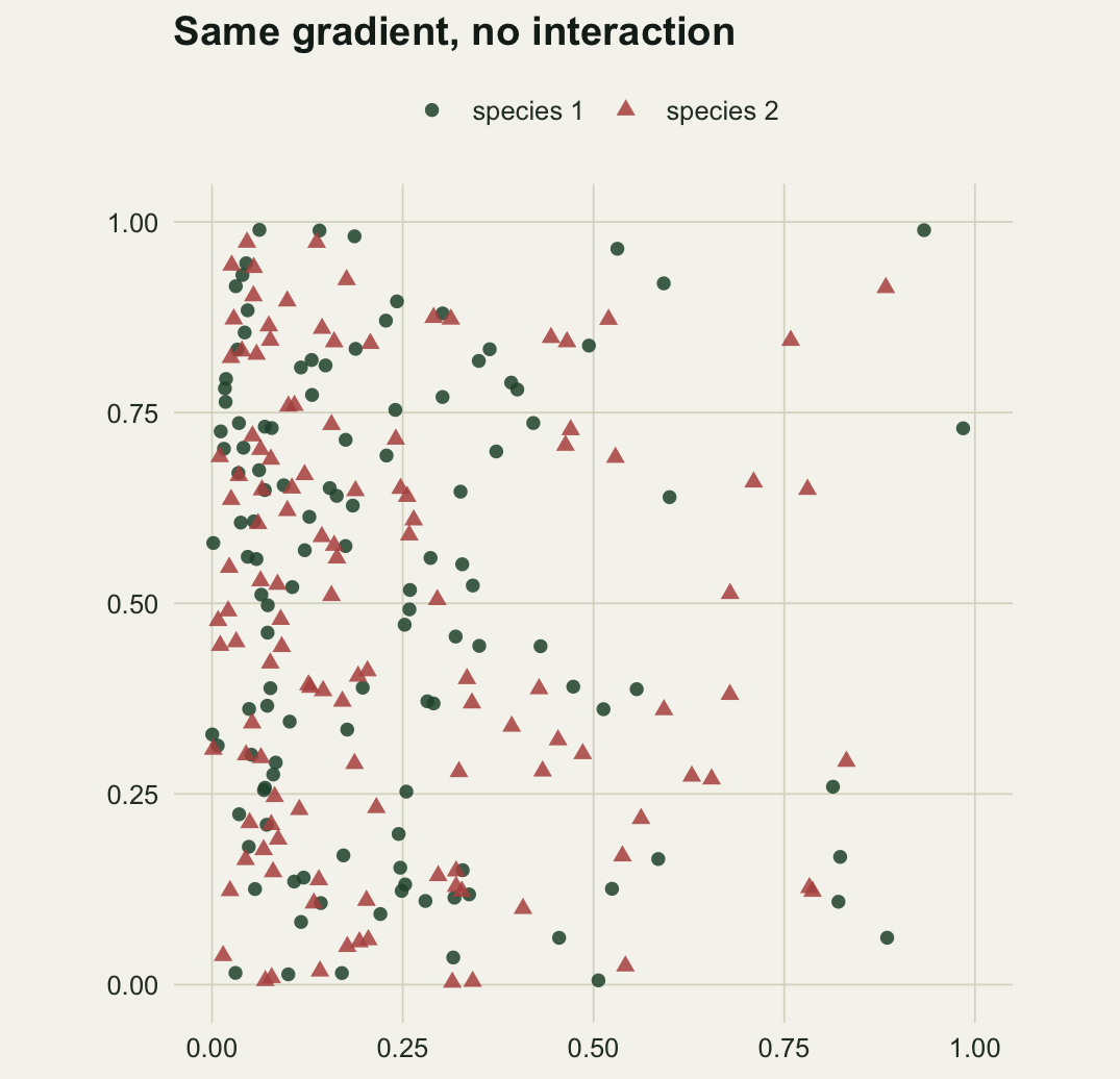
The generating process is deliberately dull: two independent inhomogeneous Poisson processes on the unit square, both with intensity falling from left to right at the same rate. No interaction of any kind. Whatever they are doing, they are doing it separately, and both are responding to the same environmental gradient, which is the situation almost every real plot is in.
```{r setup}
#| message: false
#| warning: false
library(ggplot2)

te_paper  <- "#f5f4ee"
te_ink    <- "#16241d"
te_body   <- "#2c3a31"
te_forest <- "#275139"
te_rust   <- "#b5534e"
te_gold   <- "#c9b458"
te_line   <- "#dad9ca"

theme_datasheet <- function() {
  theme_minimal(base_size = 12) +
    theme(plot.background  = element_rect(fill = te_paper, colour = NA),
          panel.background = element_rect(fill = te_paper, colour = NA),
          panel.grid.major = element_line(colour = te_line, linewidth = 0.3),
          panel.grid.minor = element_blank(),
          text             = element_text(colour = te_body),
          plot.title       = element_text(colour = te_ink, face = "bold"),
          axis.text        = element_text(colour = te_body))
}

# inhomogeneous Poisson on the unit square by rejection, intensity ~ exp(-beta x)
ipp <- function(n, beta = 4) {
  out <- matrix(NA_real_, 0, 2)
  while (nrow(out) < n) {
    m <- (n - nrow(out)) * 3
    x <- runif(m); y <- runif(m)
    keep <- runif(m) < exp(-beta * x)
    out <- rbind(out, cbind(x, y)[keep, , drop = FALSE])
  }
  out[seq_len(n), , drop = FALSE]
}

set.seed(21)
sp1 <- ipp(120)
sp2 <- ipp(120)
c(n1 = nrow(sp1), n2 = nrow(sp2),
  left_half_1 = mean(sp1[, 1] < 0.5), left_half_2 = mean(sp2[, 1] < 0.5))
```
`r sprintf("%.0f", 100 * mean(sp1[, 1] < 0.5))` per cent of the first species and `r sprintf("%.0f", 100 * mean(sp2[, 1] < 0.5))` per cent of the second sit in the left half of the plot. That is the gradient, and it is the only thing the two species have in common.
```{r fig-map}
#| fig-width: 5.6
#| fig-height: 5.4
#| fig-cap: "Two independent species on one plot, both with intensity declining from left to right. There is no interaction of any kind between them; the visual impression of association comes entirely from the shared gradient."
#| fig-alt: "A square plot with two point species drawn in different colours and shapes, both crowded towards the left edge and thinning towards the right, with no visible pairing between the two colours."
pts <- rbind(data.frame(x = sp1[, 1], y = sp1[, 2], species = "species 1"),
             data.frame(x = sp2[, 1], y = sp2[, 2], species = "species 2"))

ggplot(pts, aes(x, y, colour = species, shape = species)) +
  geom_point(size = 2, alpha = 0.85) +
  coord_fixed(xlim = c(0, 1), ylim = c(0, 1)) +
  scale_colour_manual(values = c("species 1" = te_forest, "species 2" = te_rust)) +
  scale_shape_manual(values = c(16, 17)) +
  labs(x = NULL, y = NULL, colour = NULL, shape = NULL,
       title = "Same gradient, no interaction") +
  theme_datasheet() +
  theme(legend.position = "top")
```
## The cross-K function, with an edge correction
The estimator counts, for every point of species 1, how many species 2 points fall within r, averages over the species 1 points, and divides by the intensity of species 2. Pairs near the boundary are under-counted because part of the search disc lies outside the plot, and the translation correction fixes that by weighting each pair by the reciprocal of the area of overlap between the plot and its own translate. On the unit square that weight is available in closed form.
```{r crossk}
crossK <- function(p1, p2, rs) {
  dx <- outer(p1[, 1], p2[, 1], "-")
  dy <- outer(p1[, 2], p2[, 2], "-")
  d  <- sqrt(dx^2 + dy^2)
  w  <- 1 / ((1 - abs(dx)) * (1 - abs(dy)))       # translation weight, unit square
  sapply(rs, function(r) sum(w[d <= r]) / (nrow(p1) * nrow(p2)))
}

rs    <- seq(0.02, 0.16, by = 0.01)
k_obs <- crossK(sp1, sp2, rs)
round(rbind(r = rs, observed = k_obs, csr = pi * rs^2)[, c(1, 4, 7, 11, 15)], 4)
```
Under complete independence and no gradient the cross-K would be the area of the disc, `pi * r^2`. The observed curve runs above it at every distance, reaching `r sprintf("%.4f", k_obs[rs == 0.08])` at r = 0.08 against `r sprintf("%.4f", pi * 0.08^2)` for a disc. Read naively that is mutual attraction. It is the gradient.
## Two nulls, one dataset
Both nulls are three lines. Toroidal shift displaces species 2 by a random vector and wraps it back into the square. Random labelling pools the 240 points and draws 120 of them to be species 1.
```{r nulls}
torus <- function(p, s) cbind((p[, 1] + s[1]) %% 1, (p[, 2] + s[2]) %% 1)

nsim <- 199
pool <- rbind(sp1, sp2)

set.seed(7)
k_ts <- t(replicate(nsim, crossK(sp1, torus(sp2, runif(2)), rs)))
k_rl <- t(replicate(nsim, {
  i <- sample(nrow(pool), nrow(sp1))
  crossK(pool[i, , drop = FALSE], pool[-i, , drop = FALSE], rs)
}))

round(c(observed_at_08     = k_obs[rs == 0.08],
        torus_null_mean    = mean(k_ts[, rs == 0.08]),
        labelling_null_mean = mean(k_rl[, rs == 0.08])), 4)
```
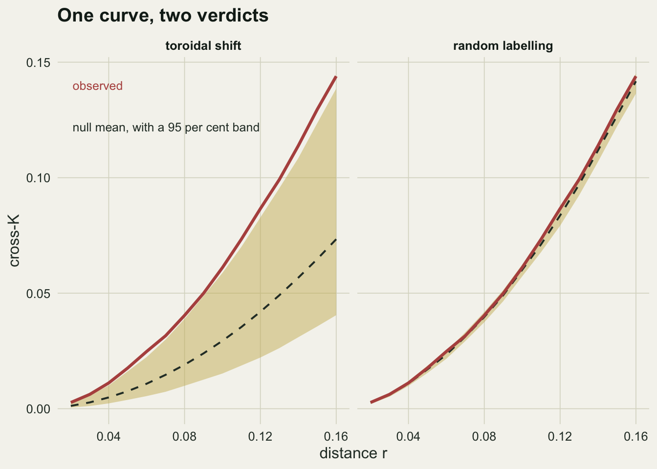
The two nulls do not even agree about what the expected cross-K is. Under toroidal shift it is `r sprintf("%.4f", mean(k_ts[, rs == 0.08]))` at r = 0.08, which is close to the `r sprintf("%.4f", pi * 0.08^2)` of a disc, because sliding one species over the other destroys the alignment of the two density gradients. Under random labelling it is `r sprintf("%.4f", mean(k_rl[, rs == 0.08]))`, which is close to the observed `r sprintf("%.4f", k_obs[rs == 0.08])`, because the pooled pattern is still crowded to the left and any two labels drawn from it will be too.
A single test over the whole distance range needs one number, not one per radius. The studentised maximum absolute deviation does it: scale the departure at each radius by the null standard deviation there, take the largest, and compare with the same quantity computed from each simulation.
```{r gdt}
gdt <- function(obs, sims) {
  mu  <- colMeans(sims)
  sdv <- apply(sims, 2, sd); sdv[sdv == 0] <- 1
  d_obs <- max(abs(obs - mu) / sdv)
  d_sim <- apply(sims, 1, function(z) max(abs(z - mu) / sdv))
  (1 + sum(d_sim >= d_obs)) / (1 + length(d_sim))
}

p_ts <- gdt(k_obs, k_ts)
p_rl <- gdt(k_obs, k_rl)
c(toroidal_shift = p_ts, random_labelling = p_rl)
```
Toroidal shift gives p = `r sprintf("%.3f", p_ts)`. Random labelling gives p = `r sprintf("%.3f", p_rl)`. There is no interaction in this dataset. One of these tests is wrong, and the plot below shows why.
```{r fig-envelopes}
#| fig-cap: "The same observed cross-K against both nulls, with pointwise 2.5 and 97.5 per cent envelopes from 199 simulations. The toroidal shift envelope sits near the disc area and the observed curve escapes it; the random labelling envelope carries the shared gradient and the observed curve sits inside."
#| fig-alt: "Two panels of cross-K against distance. In the toroidal shift panel the observed curve runs above a narrow envelope centred well below it. In the random labelling panel the same observed curve runs through the middle of an envelope that is centred on it."
band <- function(sims, nm) data.frame(
  r = rs, lo = apply(sims, 2, quantile, 0.025),
  hi = apply(sims, 2, quantile, 0.975), mid = colMeans(sims), null = nm)

lev <- c("toroidal shift", "random labelling")
env <- rbind(band(k_ts, lev[1]), band(k_rl, lev[2]))
env$null <- factor(env$null, levels = lev)
obs <- do.call(rbind, lapply(lev, function(z)
  data.frame(r = rs, k = k_obs, null = factor(z, levels = lev))))
key <- data.frame(r = 0.021, k = c(0.140, 0.122),
                  null = factor(lev[1], levels = lev),
                  lab = c("observed", "null mean, with a 95 per cent band"))

ggplot(env, aes(r)) +
  geom_ribbon(aes(ymin = lo, ymax = hi), fill = te_gold, alpha = 0.45) +
  geom_line(aes(y = mid), colour = te_body, linetype = "dashed", linewidth = 0.7) +
  geom_line(data = obs, aes(y = k), colour = te_rust, linewidth = 1.1) +
  geom_text(data = key, aes(x = r, y = k, label = lab),
            colour = c(te_rust, te_body), hjust = 0, size = 3.3) +
  facet_wrap(~ null) +
  labs(x = "distance r", y = "cross-K",
       title = "One curve, two verdicts") +
  theme_datasheet() +
  theme(strip.text = element_text(colour = te_ink, face = "bold"))
```
## Which one is right depends on what is true
A single map settles nothing, so run three worlds many times. In the first the species share a gradient and never interact. In the second they share a gradient and species 2 genuinely settles near species 1. In the third they respond to the gradient in opposite directions and still never interact.
```{r scenarios}
ipp_dir <- function(n, beta) {           # beta > 0 dense on the left, < 0 on the right
  out <- matrix(NA_real_, 0, 2); cap <- max(1, exp(-beta))
  while (nrow(out) < n) {
    m <- (n - nrow(out)) * 3; x <- runif(m); y <- runif(m)
    keep <- runif(m) < exp(-beta * x) / cap
    out <- rbind(out, cbind(x, y)[keep, , drop = FALSE])
  }
  out[seq_len(n), , drop = FALSE]
}

attracted_to <- function(p, n = 120, frac = 0.35, spread = 0.03) {
  k   <- round(n * frac)
  par <- p[sample(nrow(p), k, replace = TRUE), , drop = FALSE]
  off <- cbind(pmin(pmax(par[, 1] + rnorm(k, 0, spread), 0), 1),
               pmin(pmax(par[, 2] + rnorm(k, 0, spread), 0), 1))
  rbind(ipp(n - k), off)
}

both_p <- function(a, b, nsim = 199) {
  k  <- crossK(a, b, rs); pl <- rbind(a, b)
  ts <- t(replicate(nsim, crossK(a, torus(b, runif(2)), rs)))
  rl <- t(replicate(nsim, { i <- sample(nrow(pl), nrow(a))
                            crossK(pl[i, , drop = FALSE], pl[-i, , drop = FALSE], rs) }))
  c(ts = gdt(k, ts), rl = gdt(k, rl))
}

n_map <- 40
run <- function(gen, seed) {
  set.seed(seed)
  r <- t(replicate(n_map, gen()))
  c(torus = 100 * mean(r[, "ts"] <= 0.05), labelling = 100 * mean(r[, "rl"] <= 0.05))
}

sc <- rbind(
  "shared gradient, no interaction"    = run(function() both_p(ipp(120), ipp(120)), 4001),
  "shared gradient, real attraction"   = run(function() { a <- ipp(120)
                                              both_p(a, attracted_to(a)) }, 4002),
  "opposite gradients, no interaction" = run(function() both_p(ipp_dir(120, 4),
                                              ipp_dir(120, -4)), 4003))
round(sc, 1)
```
Read the table one row at a time, remembering that the first and third rows contain no interaction whatsoever.
Row one is the ordinary field situation, and toroidal shift calls it an association in `r sprintf("%.1f", sc[1, "torus"])` per cent of plots against a nominal 5 per cent. The reason is visible in the envelope figure: the toroidal null is not a valid null here. Both species really are independent, so the hypothesis being tested is true, but sliding an inhomogeneous pattern across the plot produces simulated maps in which the two density gradients no longer line up, and those maps are not draws from the null. Random labelling holds at `r sprintf("%.1f", sc[1, "labelling"])` per cent.
Row two puts a real attraction in, and now toroidal shift finds it in `r sprintf("%.0f", sc[2, "torus"])` per cent of plots while random labelling finds it in `r sprintf("%.1f", sc[2, "labelling"])` per cent. Random labelling is not broken here, it is weak, and the reason is structural: it conditions on the pooled set of locations, and the attraction has already happened to those locations. Permuting labels among points that are sitting in the same clumps cannot easily tell that they were sorted into the clumps by species.
Row three reverses the gradients. Now random labelling rejects in `r sprintf("%.0f", sc[3, "labelling"])` per cent of plots, and it is right to: the label really does depend on where the point is, so the labels are not exchangeable. But a reader who writes "the two species avoid each other" has said something the data does not support. They occupy different ends of an environmental gradient and never notice each other. Toroidal shift, whose null of independence is true here, comes in at `r sprintf("%.1f", sc[3, "torus"])` per cent, still above nominal but far below the rate it reaches in row one, where the shift is not a valid null.
## How strong does an attraction have to be
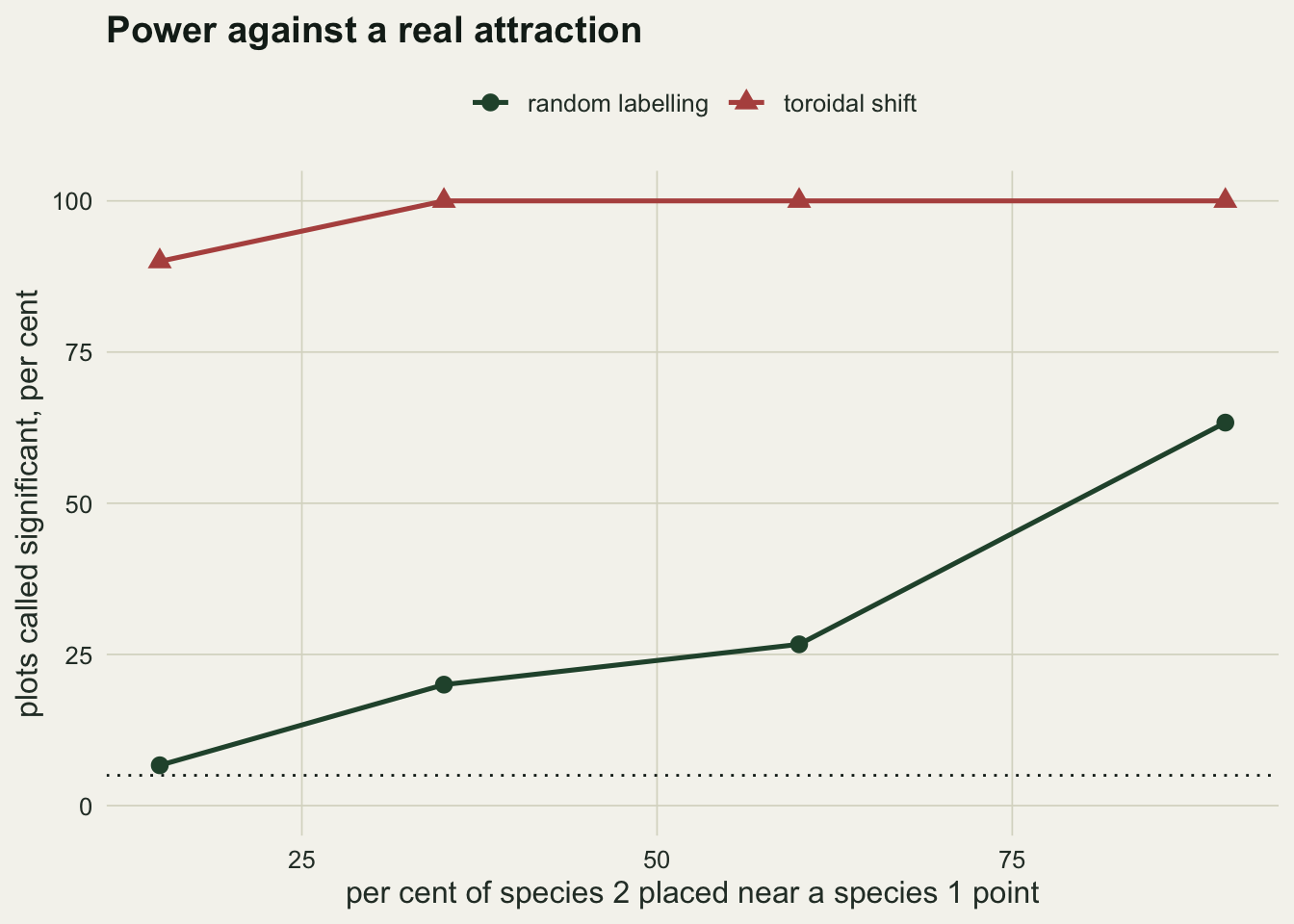
Row two is one attraction strength. Sweeping it shows where random labelling starts to see anything.
```{r strength}
strength <- do.call(rbind, lapply(c(0.15, 0.35, 0.60, 0.90), function(fr) {
  set.seed(6100)
  r <- t(replicate(30, { a <- ipp(120); both_p(a, attracted_to(a, frac = fr)) }))
  data.frame(frac = fr,
             torus     = 100 * mean(r[, "ts"] <= 0.05),
             labelling = 100 * mean(r[, "rl"] <= 0.05))
}))
strength
```
```{r fig-strength}
#| fig-cap: "Rejection rate of each null against the fraction of species 2 that is placed near a species 1 point. Thirty simulated plots per point, 199 simulations per test. The dotted line is the nominal five per cent level."
#| fig-alt: "Two rising curves against attraction strength. The toroidal shift curve starts high and saturates at one hundred per cent almost immediately, while the random labelling curve climbs slowly from near zero and is still well below one hundred at the strongest attraction."
long <- rbind(data.frame(frac = strength$frac, y = strength$torus,
                         null = "toroidal shift"),
              data.frame(frac = strength$frac, y = strength$labelling,
                         null = "random labelling"))

ggplot(long, aes(100 * frac, y, colour = null, shape = null)) +
  geom_hline(yintercept = 5, colour = te_ink, linewidth = 0.5, linetype = "dotted") +
  geom_line(linewidth = 0.9) +
  geom_point(size = 2.9) +
  scale_colour_manual(values = c("toroidal shift" = te_rust,
                                 "random labelling" = te_forest)) +
  scale_shape_manual(values = c(16, 17)) +
  scale_y_continuous(limits = c(0, 100)) +
  labs(x = "per cent of species 2 placed near a species 1 point",
       y = "plots called significant, per cent",
       colour = NULL, shape = NULL,
       title = "Power against a real attraction") +
  theme_datasheet() +
  theme(legend.position = "top")
```
At the weakest attraction random labelling is at `r sprintf("%.1f", strength$labelling[1])` per cent while toroidal shift is already at `r sprintf("%.0f", strength$torus[1])`. Even when `r sprintf("%.0f", 100 * strength$frac[nrow(strength)])` per cent of species 2 is placed within a few centimetres of a species 1 point, random labelling only reaches `r sprintf("%.0f", strength$labelling[nrow(strength)])` per cent. That is the price of a null that conditions on the locations.
## What to report
State which null you used and what it holds fixed, because the two of them are testing different sentences. Toroidal shift asks whether the two patterns are independent processes. Random labelling asks whether the species identities are exchangeable among a fixed set of locations. Neither of those is the sentence "species 1 facilitates species 2", and getting from a p value to that sentence takes an argument that the simulation cannot supply.
If the plot is heterogeneous, and it always is, toroidal shift needs replacing rather than reporting. The usual replacement estimates the intensity of each species separately and simulates from those fitted intensities, so the simulated maps keep the gradient instead of scrambling it. That test asks about interaction given the estimated habitat, and it inherits whatever the intensity estimate got wrong, which is a real cost but a smaller one than a `r sprintf("%.1f", sc[1, "torus"])` per cent false positive rate.
Random labelling is the right tool when the locations genuinely are given and only the marks are in question: dead against living stems in a mapped stand, infected against healthy, flowering against not. There the pooled pattern is not an artefact of combining two processes, it is the sampling frame.
## Honest limits
Everything here is one plot geometry, one intensity shape and one pair of sample sizes. The false positive rate of the toroidal shift grows with the strength of the shared gradient, so the number in the table is not a constant to be quoted; it is an illustration that the rate is large in an ordinary case. The direction of the failure is the part that carries over.
The three scenarios are all Poisson within species. Real mapped species clump for reasons of their own, seed dispersal and clonal spread among them, and a species that is clustered independently of any gradient breaks the toroidal null in the same way for a different reason. Fitting an intensity surface does not fix that, because the clustering is not a function of position.
The global test used above is one of several. A studentised maximum deviation is sensitive across the whole range of r, whereas a rank based global envelope is easier to draw and slightly less powerful, and a pointwise envelope with no correction at all rejects far more often than its nominal level for reasons that have nothing to do with the null model. The choice matters less than the null does, but it is not free.
Finally, the attraction simulated here is a displacement kernel, which puts species 2 near species 1 at a fixed spatial scale. Facilitation in the field acts at scales that are usually unknown, and a test tuned to the wrong range of r will miss it whichever null is behind the envelope.
## References
Lotwick HW, Silverman BW 1982 Journal of the Royal Statistical Society Series B 44(3):406-413 (10.1111/j.2517-6161.1982.tb01221.x)
Goreaud F, Pelissier R 2003 Journal of Vegetation Science 14(5):681-692 (10.1111/j.1654-1103.2003.tb02200.x)
Wiegand T, Moloney KA 2004 Oikos 104(2):209-229 (10.1111/j.0030-1299.2004.12497.x)
Baddeley A, Diggle PJ, Hardegen A, Lawrence T, Milne RK, Nair G 2014 Ecological Monographs 84(3):477-489 (10.1890/13-2042.1)
## Related tutorials
- [Ripley's K function](../ripleys-k-function/)
- [Co-occurrence null models](../co-occurrence-null-models/)
- [Measuring niche overlap](../measuring-niche-overlap/)
- [Checking a point pattern analysis](../checking-a-point-pattern-analysis/)