library(ggplot2)
library(patchwork)

te_paper  <- "#f5f4ee"
te_ink    <- "#16241d"
te_body   <- "#2c3a31"
te_forest <- "#275139"
te_rust   <- "#b5534e"
te_gold   <- "#c9b458"
te_line   <- "#dad9ca"

theme_datasheet <- function() {
  theme_minimal(base_size = 12) +
    theme(plot.background  = element_rect(fill = te_paper, colour = NA),
          panel.background = element_rect(fill = te_paper, colour = NA),
          panel.grid.major = element_line(colour = te_line, linewidth = 0.3),
          panel.grid.minor = element_blank(),
          text             = element_text(colour = te_body),
          plot.title       = element_text(colour = te_ink, face = "bold"),
          plot.subtitle    = element_text(colour = te_body),
          axis.text        = element_text(colour = te_body))
}Emulating a slow simulation model
R
simulation
Gaussian processes
computer experiments
ecology tutorial
A Gaussian process emulator from 64 runs of a harvest model in R: grid against Latin hypercube, leave-one-out checks, and a jitter that sets the coverage.
A harvest model for a game population has three parameters nobody can pin down from the field: the intrinsic growth rate, the harvest rate a management plan might set, and the shape of density dependence. The manager wants the stock left after twenty five years across the whole plausible box of those three, and the modeller has a simulator that answers one parameter combination at a time. If the simulator is an individual based model with spatial movement and a demographic lottery, one run can take an hour. A thousand runs across the box is six weeks of a workstation, and the plan is due on Friday.
The standard answer is an emulator: run the simulator at a few dozen carefully placed parameter combinations, fit a statistical surface through the outputs, and ask the surface instead of the simulator. The surface usually used is a Gaussian process, and this site already has one. The post on Gaussian process regression fits a process to noisy field observations along one gradient, estimates a noise variance, and shows that the length-scale is only weakly identified by one sample. An emulator is a different problem that uses the same algebra. The simulator here is deterministic, so there is no noise to smooth: run it twice at the same parameters and the answer is identical, and the fitted surface is meant to pass through every run. The question stops being how much to smooth and becomes how many runs to buy and where to put them.
The word emulated also appears in the stock assessment checks, in a different sense. There the assessment inside a closed management loop is replaced by a lognormal error with a measured standard deviation and autocorrelation, because refitting a likelihood inside 400 replicates of fifty years costs minutes for no extra realism. That stand-in has a form chosen in advance and two numbers measured once. The emulator in this post learns its form from the runs themselves, and it reports its own uncertainty at every parameter combination it was not run at. Whether that uncertainty can be believed is one of the things measured below.
A simulator is a function
The simulator is a theta-logistic population with proportional harvest, integrated by a fourth order Runge-Kutta scheme with a step of a fiftieth of a year. Density is scaled so that carrying capacity is one, and every run starts at a tenth of carrying capacity and returns the density after twenty five years. A differential equation this small runs in microseconds, which is what makes the measurements in this post possible; the rule adopted here is to pretend otherwise and count every call. A counter inside the function records runs, and each section below reports what it spent.
The parameter box is fixed before anything is fitted: growth rate from 0.5 to 1, harvest rate from 0 to 0.3, and the density dependence exponent from 0.5 to 3. Harvest never reaches growth anywhere in this box, so every population persists; a wider box that crosses the collapse edge comes at the end. All inputs are rescaled to the unit cube before the emulator sees them, so a length-scale of one means the whole width of a parameter range.
box_lo <- c(r = 0.5, h = 0.0, theta = 0.5)   # lower corner of the parameter box
box_hi <- c(r = 1.0, h = 0.3, theta = 3.0)   # upper corner
n_years <- 25; dt_step <- 0.02; n_start <- 0.1
run_count <- 0

to_natural <- function(u, lo, hi) sweep(sweep(u, 2, hi - lo, "*"), 2, lo, "+")

simulator <- function(u, lo = box_lo, hi = box_hi) {
  u <- matrix(u, ncol = 3)
  run_count <<- run_count + nrow(u)            # every row is one expensive run
  pars <- to_natural(u, lo, hi)
  r <- pars[, 1]; h <- pars[, 2]; th <- pars[, 3]
  growth <- function(N) r * N * (1 - N^th) - h * N
  N <- rep(n_start, nrow(u))
  for (s in seq_len(round(n_years / dt_step))) {
    k1 <- growth(N); k2 <- growth(N + dt_step / 2 * k1)
    k3 <- growth(N + dt_step / 2 * k2); k4 <- growth(N + dt_step * k3)
    N <- N + dt_step / 6 * (k1 + 2 * k2 + 2 * k3 + k4)
  }
  N
}
n_test <- 2000
set.seed(20821)
x_test <- matrix(runif(n_test * 3), ncol = 3)
y_test <- simulator(x_test)
test_sd <- sd(y_test); test_min <- min(y_test); test_max <- max(y_test)
runs_test <- run_count
The 2000 runs above are the held-out test set, drawn uniformly over the box and never shown to any emulator. In a real study nobody could afford them; here they are the reference every accuracy and coverage figure is measured against. Across the test set the stock after twenty five years runs from 0.222 to 1.000 of carrying capacity, with a standard deviation of 0.124. That standard deviation is the error of the laziest possible emulator, one that always answers with the mean, and every error below can be read against it.
slice_n <- 60
slice_u <- as.matrix(expand.grid(r = seq(0, 1, length.out = slice_n),
                                 h = seq(0, 1, length.out = slice_n), theta = 0.5))
slice_tab <- data.frame(to_natural(slice_u, box_lo, box_hi), N = simulator(slice_u))
ggplot(slice_tab, aes(r, h)) +
  geom_raster(aes(fill = N)) +
  geom_contour(aes(z = N), colour = te_paper, linewidth = 0.3, breaks = seq(0.1, 1, 0.1)) +
  scale_fill_gradient(low = te_forest, high = te_gold, name = "stock after\n25 years") +
  labs(x = "intrinsic growth rate r", y = "harvest rate h",
       title = "One slice of the simulator", subtitle = "density dependence exponent at 1.75") +
  theme_datasheet()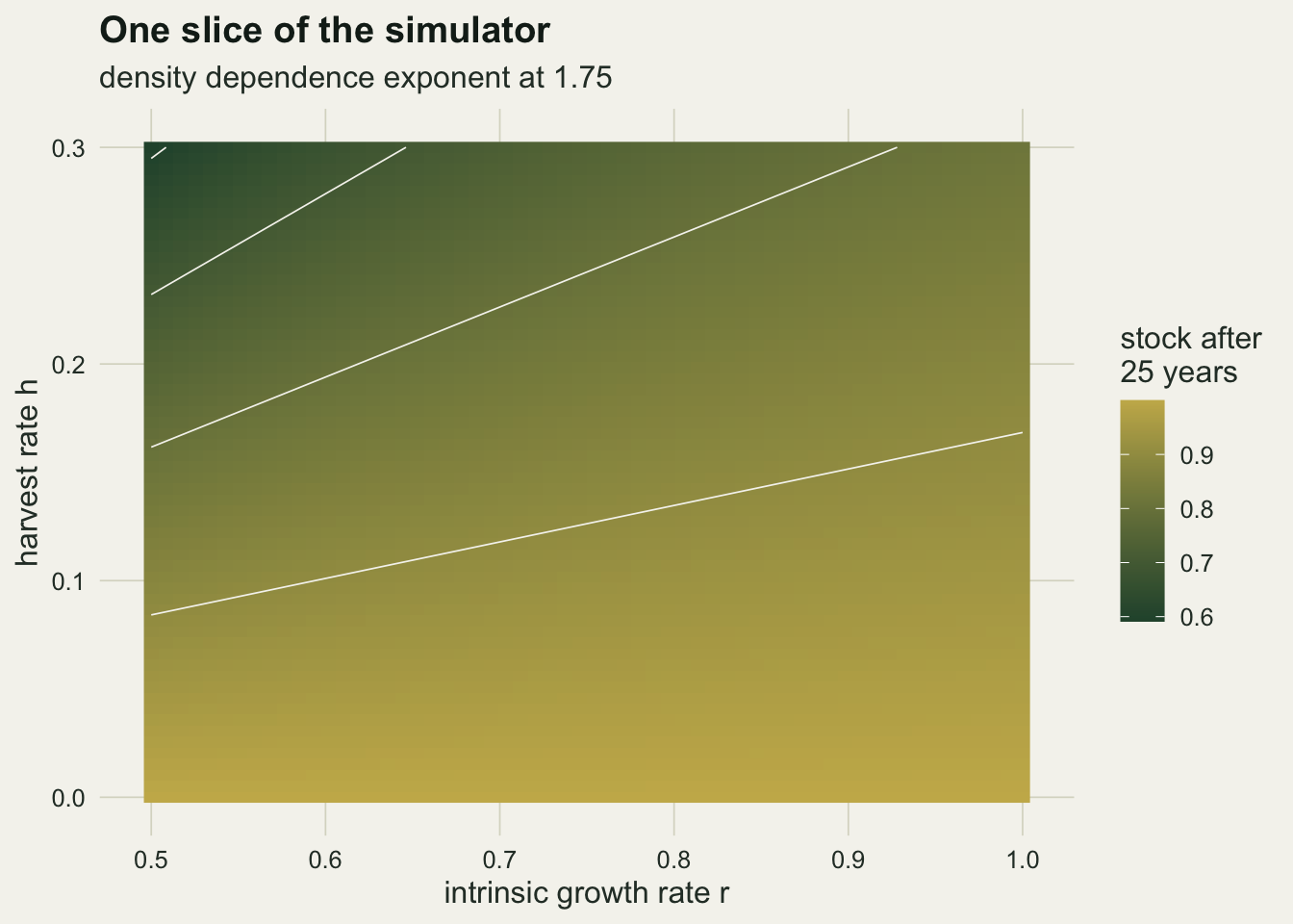
The slice spends another 3600 runs to draw a picture nobody would have in practice. It shows a smooth surface: the stock falls with harvest and rises with growth, and the contours are nearly straight lines fanning out from the lower left, because what matters is roughly the ratio of the two. Smooth is the case a Gaussian process emulator is built for.
Sixty four runs and a Gaussian process
A Latin hypercube with a budget of runs cuts the range of every input into that many equal strata and puts exactly one run in each stratum of each input, pairing the strata across inputs by independent random permutations, as McKay, Beckman and Conover defined it. The code below is that definition and nothing more: a random permutation of stratum labels for each column and a uniform position inside each stratum.
The emulator follows Sacks, Welch, Mitchell and Wynn: a constant mean, a process variance, and a Gaussian correlation with a separate length-scale for each input. Given the length-scales, the constant and the process variance have closed form maximum likelihood estimates, so they are profiled out and only the three log length-scales go to optim. Working on the log scale keeps them positive and makes a change from 0.1 to 0.2 as large a step as one from 1 to 2. Three starting points guard against a local optimum, and bounds keep the search between a fiftieth of the box and twenty times it. The predictive variance includes the extra term for having estimated the constant, which is the kriging mean squared error of Sacks and colleagues. A fixed jitter of one in a hundred million is added to the diagonal of the correlation matrix so that the Cholesky factorisation does not fail. That constant was set before anything was fitted, and it turns out not to be a purely numerical detail, so the coverage section refits the emulators at other jitters. The same functions also carry a Matern 5/2 correlation, which assumes a surface that is twice differentiable rather than infinitely smooth; everything up to the coverage section uses the Gaussian one.
lhs_design <- function(n, d = 3) {
  sapply(seq_len(d), function(j) (sample.int(n) - runif(n)) / n)
}
jitter_fixed <- 1e-8
corr_mat <- function(A, B, ell, kernel = "gauss") {
  d2 <- Reduce(`+`, lapply(seq_along(ell), function(j) outer(A[, j], B[, j], "-")^2 / ell[j]^2))
  if (kernel == "gauss") return(exp(-d2))
  dist5 <- sqrt(5 * d2)                         # Matern 5/2
  (1 + dist5 + dist5^2 / 3) * exp(-dist5)
}
# negative profile log likelihood: constant mean and process variance profiled out
nll_profile <- function(par, X, y, kernel = "gauss", nug = jitter_fixed) {
  ell <- exp(par[1:3]); if (length(par) > 3) nug <- exp(par[4])
  n <- nrow(X)
  R <- corr_mat(X, X, ell, kernel); diag(R) <- 1 + nug
  ch <- tryCatch(chol(R), error = function(e) NULL)
  if (is.null(ch)) return(1e10)
  solve_r <- function(b) backsolve(ch, forwardsolve(t(ch), b))
  ri_1 <- solve_r(rep(1, n)); beta <- sum(solve_r(y)) / sum(ri_1)
  resid <- y - beta
  s2 <- sum(resid * solve_r(resid)) / n
  0.5 * n * log(s2) + sum(log(diag(ch)))
}
ell_bounds <- log(c(0.02, 20))
fit_gp <- function(X, y, est_nugget = FALSE, kernel = "gauss", nug = jitter_fixed) {
  starts <- list(log(rep(0.5, 3)), log(rep(0.2, 3)), log(rep(2, 3)))
  lower_b <- rep(ell_bounds[1], 3); upper_b <- rep(ell_bounds[2], 3)
  if (est_nugget) {
    starts <- lapply(starts, function(s0) c(s0, log(1e-4)))
    lower_b <- c(lower_b, log(1e-12)); upper_b <- c(upper_b, log(1e-1))
  }
  best <- NULL
  for (s0 in starts) {
    o <- optim(s0, nll_profile, X = X, y = y, kernel = kernel, nug = nug,
               method = "L-BFGS-B", lower = lower_b, upper = upper_b)
    if (is.null(best) || o$value < best$value) best <- o
  }
  best
}
predict_gp <- function(par, X, y, Xnew, kernel = "gauss", nug = jitter_fixed) {
  ell <- exp(par[1:3]); if (length(par) > 3) nug <- exp(par[4])
  n <- nrow(X)
  R <- corr_mat(X, X, ell, kernel); diag(R) <- 1 + nug; ch <- chol(R)
  solve_r <- function(b) backsolve(ch, forwardsolve(t(ch), b))
  ri_1 <- solve_r(rep(1, n)); beta <- sum(solve_r(y)) / sum(ri_1)
  resid <- y - beta; ri_res <- solve_r(resid); s2 <- sum(resid * ri_res) / n
  r_new <- corr_mat(Xnew, X, ell, kernel)
  mu <- beta + as.vector(r_new %*% ri_res)
  half <- forwardsolve(t(ch), t(r_new))
  u_term <- 1 - as.vector(r_new %*% ri_1)
  v <- s2 * (1 - colSums(half^2) + u_term^2 / sum(ri_1))
  list(mu = mu, sd = sqrt(pmax(v, 0)), s2 = s2, beta = beta)
}
n_design <- 64
set.seed(4107)
x_one <- lhs_design(n_design)
strata_ok <- all(apply(x_one, 2, function(col) all(sort(ceiling(col * n_design)) == seq_len(n_design))))
run_count <- 0
y_one <- simulator(x_one)
fit_one <- fit_gp(x_one, y_one)
ell_one <- exp(fit_one$par)
pred_one <- predict_gp(fit_one$par, x_one, y_one, x_test)
err_one <- y_test - pred_one$mu
rmse_one <- sqrt(mean(err_one^2)); maxerr_one <- max(abs(err_one))
at_design <- predict_gp(fit_one$par, x_one, y_one, x_one)
interp_gap <- max(abs(at_design$mu - y_one)); sd_at_design <- max(at_design$sd)
cond_one <- kappa(corr_mat(x_one, x_one, ell_one), exact = TRUE)
fit_nug <- fit_gp(x_one, y_one, est_nugget = TRUE)
nug_hat <- exp(fit_nug$par[4]); nll_gain <- fit_one$value - fit_nug$value
nug_sd <- sqrt(nug_hat * predict_gp(fit_nug$par, x_one, y_one, x_one[1:2, ])$s2)
pred_nug <- predict_gp(fit_nug$par, x_one, y_one, x_test)
rmse_nug <- sqrt(mean((y_test - pred_nug$mu)^2))
s2_one <- pred_one$s2; out_var <- var(y_test)
runs_one <- run_count
The design check returns TRUE: every one of the 64 strata of every input holds exactly one run. The fit cost 64 simulator runs. The estimated length-scales are 2.42 for growth, 2.18 for harvest and 0.76 for the density dependence exponent, all well inside the bounds and all measured in widths of the box. The first two are longer than the box itself, which is what the slice showed: across the range of growth and harvest the output bends gently. The exponent does more work over a shorter distance.
On the 2000 held-out runs the emulator has a root mean squared error of 0.0021 of carrying capacity, which is 1.7 per cent of the standard deviation of the output, and its worst single error is 0.0223. At the design points it returns the simulator output to within 1.5e-04, with a predictive standard deviation no larger than 1.1e-04. Those two numbers are not zero because of the jitter, and the jitter matters more than its size suggests: with length-scales longer than the box the correlation matrix has a condition number of 1.7e+11, so a diagonal addition of one in a hundred million is amplified into disagreements of that order at the runs themselves. That miss is still 14 times smaller than the error between the runs. The jitter is added to a correlation, so in output units it behaves like a noise variance of the jitter times the process variance, and the fitted process variance is 1.23 where the output itself has a variance of 0.0154. When that ratio is large the jitter stops being negligible, which the next section shows for the grid.
The nugget can also be estimated rather than fixed, which is what a noisy regression would do. Given the chance, maximum likelihood puts it at 1.8e-08 of the process variance, a noise standard deviation of 1.3e-04 in output units. That is the same order as the fixed jitter, and it improves the log likelihood by 0.14. The test error with the estimated nugget is 0.00210 against 0.00207 with it fixed. The data contain no noise, and the likelihood cannot tell a nugget apart from the numerical floor it sits on: estimating the nugget swaps one small constant for another of the same size rather than removing the choice. That is the practical difference from the regression post: there the noise variance was a quantity of interest, and here an estimated nugget far above jitter size would be a warning that the simulator is not as deterministic as believed, or that the surface is rougher than a Gaussian correlation can follow.
Same budget, three designs
A budget of 64 runs in three dimensions can be spent three obvious ways: a regular grid of four levels per input, 64 points drawn uniformly at random, or a Latin hypercube. The grid is the design a person draws without thinking, with levels at both ends of each range and two in between. The random and Latin hypercube designs are redrawn 40 times each, a number fixed before any design was scored, and every emulator is fitted and scored in the same way on the same test set.
grid_levels <- seq(0, 1, length.out = 4)
x_grid <- as.matrix(expand.grid(grid_levels, grid_levels, grid_levels))
n_rep <- 40   # fixed before any design was scored
set.seed(7730)
z_store <- list(); design_store <- list()
# leave-one-out error: refit nothing, drop each run in turn and predict it from the rest
loo_rmse <- function(par, X, y, kernel = "gauss") {
  sqrt(mean(vapply(seq_len(nrow(X)), function(i)
    y[i] - predict_gp(par, X[-i, ], y[-i], X[i, , drop = FALSE], kernel)$mu, 0)^2))
}
score_keep <- function(X, label, matern = TRUE, loo = TRUE) {
  y <- simulator(X)
  design_store[[label]] <<- c(design_store[[label]], list(list(X = X, y = y)))
  f <- fit_gp(X, y); p <- predict_gp(f$par, X, y, x_test)
  z_store[[paste("gauss", label)]] <<- c(z_store[[paste("gauss", label)]], (y_test - p$mu) / p$sd)
  rmse_m <- NA
  if (matern) {
    fm <- fit_gp(X, y, kernel = "matern"); pm <- predict_gp(fm$par, X, y, x_test, "matern")
    z_store[[paste("matern", label)]] <<- c(z_store[[paste("matern", label)]], (y_test - pm$mu) / pm$sd)
    rmse_m <- sqrt(mean((y_test - pm$mu)^2))
  }
  c(rmse = sqrt(mean((y_test - p$mu)^2)), mean_sd = sqrt(mean(p$sd^2)),
    loo = if (loo) loo_rmse(f$par, X, y) else NA,
    gap = max(abs(predict_gp(f$par, X, y, X)$mu - y)), s2 = p$s2,
    ell_max = max(exp(f$par)), rmse_m = rmse_m)
}
run_count <- 0
res_grid <- score_keep(x_grid, "regular grid")
res_lhs <- t(replicate(n_rep, score_keep(lhs_design(n_design), "Latin hypercube")))
res_rand <- t(replicate(n_rep, score_keep(matrix(runif(n_design * 3), ncol = 3), "random")))
runs_designs <- run_count
design_tab <- data.frame(
  design = factor(rep(c("regular grid", "random", "Latin hypercube"), c(1, n_rep, n_rep)),
                  levels = c("regular grid", "random", "Latin hypercube")),
  rmse = c(res_grid["rmse"], res_rand[, "rmse"], res_lhs[, "rmse"]))
rmse_lhs <- mean(res_lhs[, "rmse"]); mcse_lhs <- sd(res_lhs[, "rmse"]) / sqrt(n_rep)
rmse_rand <- mean(res_rand[, "rmse"]); mcse_rand <- sd(res_rand[, "rmse"]) / sqrt(n_rep)
rmse_grid <- unname(res_grid["rmse"])
grid_ratio <- rmse_grid / rmse_lhs
worst_lhs <- max(res_lhs[, "rmse"]); worst_rand <- max(res_rand[, "rmse"])
rand_worse_share <- mean(outer(res_rand[, "rmse"], res_lhs[, "rmse"], ">"))
f_grid <- fit_gp(x_grid, design_store[["regular grid"]][[1]]$y); ell_grid <- exp(f_grid$par)
ell_cap <- exp(ell_bounds[2])
gap_grid <- unname(res_grid["gap"]); gap_lhs_max <- max(res_lhs[, "gap"])
s2_grid <- unname(res_grid["s2"]); s2_lhs_max <- max(res_lhs[, "s2"])
loo_grid <- unname(res_grid["loo"]); loo_lhs <- mean(res_lhs[, "loo"]); loo_lhs_max <- max(res_lhs[, "loo"])
loo_rand_max <- max(res_rand[, "loo"])
cor_loo_test <- cor(res_lhs[, "loo"], res_lhs[, "rmse"])
ellmax_lhs <- max(c(res_lhs[, "ell_max"], res_rand[, "ell_max"]))
rmse_m_grid <- unname(res_grid["rmse_m"]); rmse_m_lhs <- mean(res_lhs[, "rmse_m"])
rmse_m_rand <- mean(res_rand[, "rmse_m"])
msd_grid <- unname(res_grid["mean_sd"]); msd_lhs <- mean(res_lhs[, "mean_sd"])
sd_ratio_grid <- rmse_grid / msd_grid
sd_ratio_lhs <- mean(res_lhs[, "rmse"] / res_lhs[, "mean_sd"])
gap_over_test_n <- sum(c(res_lhs[, "gap"] > res_lhs[, "rmse"], res_rand[, "gap"] > res_rand[, "rmse"]))
s2_ratio_min <- min(c(res_lhs[, "s2"], res_rand[, "s2"])) / out_var
The grid emulator has a test error of 0.0097. The Latin hypercube emulators average 0.0029 with a Monte Carlo standard error of 0.00013, so the grid is 3.4 times worse than the typical Latin hypercube for the same 64 runs, and worse than the worst of the 40 hypercubes, which reached 0.0051. The ranking does not depend on the correlation function: refitted with a Matern 5/2 correlation, the grid reaches 0.0113 against an average of 0.0038 for the hypercubes. The grid is not slower; it is less accurate.
The reason is visible in the left panel of the figure. Seen along any pair of inputs, the grid stacks its runs four deep on sixteen positions, and along any single input it has only four distinct values. The Latin hypercube shows sixty four distinct values on every axis. When an input changes the output over a short length-scale, as the density dependence exponent does here, four values of it are four values, however many runs sit on each.
The result that did not match the design literature’s usual message is the comparison with random points. Random designs average 0.0028 with a Monte Carlo standard error of 0.00013, indistinguishable from the Latin hypercube, and a random design beats a Latin hypercube in 51 per cent of all random against hypercube pairings. The worst random design reached 0.0051, the same as the worst hypercube. McKay and colleagues showed that Latin hypercube sampling estimates the mean of an output with less variance than random sampling when the output is monotone in each input, and stratifying each input separately is what delivers that. An emulator’s error depends on how far a test point can be from its nearest run in all three dimensions at once, and a plain Latin hypercube does nothing to control that distance: a permutation that lines the runs up along a diagonal is a valid hypercube. With sixty four runs in three dimensions, random points already cover each axis evenly enough that stratifying it adds little. What protected the emulator was avoiding the grid, not choosing the hypercube.
proj_tab <- rbind(
  data.frame(design = "regular grid", r = x_grid[, 1], h = x_grid[, 2]),
  data.frame(design = "Latin hypercube", r = x_one[, 1], h = x_one[, 2]))
proj_tab$design <- factor(proj_tab$design, levels = c("regular grid", "Latin hypercube"))
p_proj <- ggplot(proj_tab, aes(r, h)) +
  geom_point(colour = te_forest, size = 1.6, alpha = 0.7) +
  facet_wrap(~ design, ncol = 1) +
  coord_equal() +
  labs(x = "growth rate, scaled", y = "harvest rate, scaled",
       title = "Runs seen from above") +
  theme_datasheet()
p_rmse <- ggplot(design_tab, aes(design, rmse)) +
  geom_jitter(width = 0.12, height = 0, colour = te_forest, alpha = 0.6, size = 1.8) +
  stat_summary(fun = mean, geom = "point", shape = 23, size = 3.5, fill = te_gold, colour = te_ink) +
  scale_y_log10() +
  labs(x = NULL, y = "test RMSE, fraction of carrying capacity",
       title = "Same budget, three designs", subtitle = "diamonds: mean over the designs drawn") +
  theme_datasheet()
p_proj + p_rmse + plot_layout(widths = c(1, 1.6)) + plot_annotation(theme = theme_datasheet())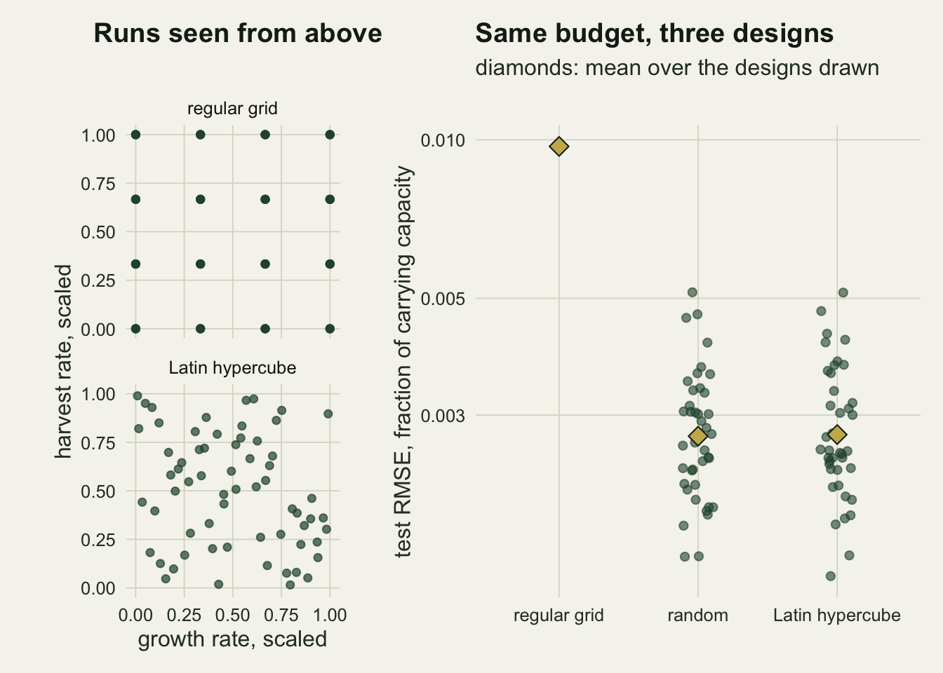
The grid fit also shows trouble without a single test run, for anyone who looks. At its own sixty four runs it misses the simulator output by up to 0.0151, more than its error on the test set, where the largest miss among the forty hypercube fits is 0.0030. Its fitted process variance is 4248 for an output whose variance is 0.0154 (the largest among the hypercube fits is 70), and its growth length-scale is 19.0 box widths against a search cap of 20, where no random or hypercube fit went above 9.8. With a process variance that large, the jitter of one in a hundred million acts as a noise standard deviation of 0.0065 in output units, and the surface no longer passes through the runs.
The standard emulator check needs no extra runs either. Leave-one-out prediction drops each run in turn and predicts it from the other sixty three at the fitted length-scales. The grid’s leave-one-out error is 0.0112, against an average of 0.0025 for the hypercubes, 0.0062 for the worst of them and at most 0.0060 for a random design. The grid is caught from its own runs. Leave-one-out is much weaker at ranking designs that are all reasonable: across the forty hypercubes its correlation with the test error is 0.11.
The emulator’s own predictive standard deviation, averaged over the box, is 0.0037 for the grid against 0.0013 for the average hypercube, so that number also points the right way. It is not large enough, though: the grid’s actual error is 2.66 times its own average standard deviation, and the hypercube’s is 2.25 times. Both emulators are overconfident, which is the subject of the section after next.
How many runs to buy
The budget question is the one a modeller actually faces. Loeppky, Sacks and Welch suggested ten runs per input as a starting point, which here would be thirty. The same Latin hypercube construction was run at four budgets, with twenty designs at each new budget and the forty from above reused at sixty four.
budgets <- c(16, 32, 64, 128)
n_rep_budget <- 20
set.seed(3391)
run_count <- 0
budget_tab <- do.call(rbind, lapply(budgets, function(nb) {
  sc <- if (nb == n_design) res_lhs else
    t(replicate(n_rep_budget, score_keep(lhs_design(nb), paste("Latin hypercube", nb),
                                         matern = nb < 128, loo = FALSE)))   # Matern skipped at 128 for knit time
  data.frame(runs = nb, rmse = sc[, "rmse"], mean_sd = sc[, "mean_sd"])
}))
runs_budget <- run_count
budget_mean <- aggregate(cbind(rmse, mean_sd) ~ runs, data = budget_tab, FUN = mean)
b_rmse <- function(nb) budget_mean$rmse[budget_mean$runs == nb]
b_sd <- function(nb) sd(budget_tab$rmse[budget_tab$runs == nb])
slope_fit <- unname(coef(lm(log(rmse) ~ log(runs), data = budget_mean))[2])
share32_above <- mean(budget_tab$rmse[budget_tab$runs == 32] > 0.01)
This section spent 3520 runs. The average test error is 0.0284 at sixteen runs, 0.0090 at thirty two, 0.0029 at sixty four and 0.0010 at one hundred and twenty eight. As fractions of the output standard deviation those are 22.9, 7.3, 2.3 and 0.8 per cent. A line through the logarithms has a slope of -1.60, so each doubling of the budget divided the error by about 3.0 over this range. For a surface this smooth the ten per input rule is adequate: thirty two runs bring the average error below a hundredth of carrying capacity, though 40 per cent of those designs stay above it. That rate belongs to this simulator and would be slower for a rougher one; the point of measuring it is that it can be measured, from a small pilot design and a handful of held-out runs, before the main budget is committed.
Does the emulator know its own error
An emulator that is going to replace a simulator in a decision has to carry its uncertainty with it. The predictive standard deviation promises that about ninety five per cent of the held-out outputs fall within 1.96 standard deviations of the emulator mean. The standardised errors of every fit above were stored, so the promise can be checked at several levels on runs no emulator saw.
nominal <- c(0.5, 0.8, 0.9, 0.95, 0.99)
cover_of <- function(z) vapply(nominal, function(a) mean(abs(z) < qnorm(1 - (1 - a) / 2)), 0)
cover_tab <- do.call(rbind, lapply(names(z_store), function(key)
  data.frame(kernel = sub(" .*", "", key), design = sub("^[a-z]+ ", "", key),
             nominal = nominal, empirical = cover_of(z_store[[key]]))))
cov95 <- function(lab, kern = "gauss") {
  cover_tab$empirical[cover_tab$design == lab & cover_tab$kernel == kern & cover_tab$nominal == 0.95]
}
z_scale <- sd(z_store[["gauss Latin hypercube"]])
z_scale_m <- sd(z_store[["matern Latin hypercube"]])
cov_g <- cover_tab$empirical[cover_tab$kernel == "gauss" & cover_tab$nominal == 0.95]
cov_m <- cover_tab$empirical[cover_tab$kernel == "matern" & cover_tab$nominal == 0.95]
spear_one <- cor(abs(err_one), pred_one$sd, method = "spearman")
top_decile <- pred_one$sd >= quantile(pred_one$sd, 0.9)
err_share_top <- sum(err_one[top_decile]^2) / sum(err_one^2)
v_ratio_med <- median(pred_one$sd^2 / s2_one)   # predictive variance in units of the process variance
With the Gaussian correlation and the jitter used so far, the nominal ninety five per cent interval covers 76.5 per cent of held-out runs for the sixty four run hypercubes, 75.8 per cent for the random designs and 66.3 per cent for the grid. With more runs the shortfall shrinks without closing: 65.9 per cent at sixteen runs and 83.6 per cent at one hundred and twenty eight. The standard deviation of the standardised errors for the sixty four run hypercubes is 2.05, where a calibrated emulator would give one. Every Gaussian emulator whose coverage was checked here claims more accuracy than it has.
The standard deviation is much better at ranking than at scaling. Across the held-out runs of the single emulator fitted above, the rank correlation between the absolute error and the predictive standard deviation is 0.67, and the tenth of the box where the emulator reported the largest standard deviation holds 69 per cent of the total squared error. The emulator knows where it is weak. It does not know by how much.
# integrate over the log length-scales: flat prior inside the bounds, constant and variance integrated out
log_marg <- function(par, X, y) {
  if (any(par < ell_bounds[1] | par > ell_bounds[2])) return(-Inf)
  n <- nrow(X); R <- corr_mat(X, X, exp(par)); diag(R) <- 1 + jitter_fixed
  ch <- tryCatch(chol(R), error = function(e) NULL)
  if (is.null(ch)) return(-Inf)
  solve_r <- function(b) backsolve(ch, forwardsolve(t(ch), b))
  ri_1 <- solve_r(rep(1, n)); beta <- sum(solve_r(y)) / sum(ri_1); resid <- y - beta
  -sum(log(diag(ch))) - 0.5 * log(sum(ri_1)) - 0.5 * (n - 1) * log(sum(resid * solve_r(resid)))
}
set.seed(918)
n_iter <- 6000; n_burn <- 1000; n_thin <- 50
current <- fit_one$par; lp_current <- log_marg(current, x_one, y_one); draws <- NULL
for (it in seq_len(n_iter)) {
  proposal <- current + rnorm(3, 0, 0.15)
  lp_proposal <- log_marg(proposal, x_one, y_one)
  if (log(runif(1)) < lp_proposal - lp_current) { current <- proposal; lp_current <- lp_proposal }
  if (it > n_burn && it %% n_thin == 0) draws <- rbind(draws, current)
}
# Student t predictive: the process variance divided by n - 1 instead of n
t_pit <- function(p) pt((y_test - p$mu) / (p$sd * sqrt(n_design / (n_design - 1))), n_design - 1)
pit_bayes <- rowMeans(sapply(seq_len(nrow(draws)), function(k)
  t_pit(predict_gp(draws[k, ], x_one, y_one, x_test))))
cov_plug <- mean(abs(err_one) < qnorm(0.975) * pred_one$sd)
cov_t <- mean(abs(t_pit(pred_one) - 0.5) < 0.475)
cov_bayes <- mean(abs(pit_bayes - 0.5) < 0.475)
ell_post <- apply(exp(draws), 2, quantile, c(0.05, 0.95))
The first suspect is the length-scales, which were estimated and then treated as known. The predictive variance allows for not knowing the output between runs and for not knowing the constant mean, but not for the length-scales. That was measured on the single hypercube emulator fitted earlier, whose plug-in interval covers 72.6 per cent. A Student t predictive, which divides by the degrees of freedom left after estimating the constant, covers 73.5 per cent. Averaging that t predictive over 100 posterior draws of the three log length-scales (flat prior inside the bounds, random walk Metropolis, constant and process variance integrated out) covers 78.8 per cent. The central ninety per cent of the posterior runs from 2.00 to 3.08 box widths for growth, 1.75 to 2.82 for harvest and 0.67 to 0.87 for the exponent. Sixty four noise-free runs pin the length-scales down more tightly than the single field gradient of the regression post, and integrating over them closes only a small part of the gap.
jitters <- c(1e-10, 1e-8, 1e-6)
n_sweep <- 20   # the first twenty of the forty hypercubes, for knit time
lhs_runs <- design_store[["Latin hypercube"]][seq_len(n_sweep)]
sweep_tab <- do.call(rbind, lapply(c("gauss", "matern"), function(k) do.call(rbind, lapply(jitters, function(jt) {
  if (jt == jitter_fixed) {
    z <- z_store[[paste(k, "Latin hypercube")]][seq_len(n_sweep * n_test)]
    err <- mean(res_lhs[seq_len(n_sweep), if (k == "gauss") "rmse" else "rmse_m"])
  } else {
    fits <- lapply(lhs_runs, function(d) {
      f <- fit_gp(d$X, d$y, kernel = k, nug = jt); p <- predict_gp(f$par, d$X, d$y, x_test, k, jt)
      list(z = (y_test - p$mu) / p$sd, rmse = sqrt(mean((y_test - p$mu)^2)))
    })
    z <- unlist(lapply(fits, `[[`, "z")); err <- mean(vapply(fits, `[[`, 0, "rmse"))
  }
  data.frame(kernel = k, jitter = jt, nominal = nominal, empirical = cover_of(z), rmse = err)
}))))
sw95 <- function(k, jt) sweep_tab$empirical[sweep_tab$kernel == k & sweep_tab$jitter == jt & sweep_tab$nominal == 0.95]
sw_rmse <- function(k, jt) sweep_tab$rmse[sweep_tab$kernel == k & sweep_tab$jitter == jt][1]
fit_nug_m <- fit_gp(x_one, y_one, est_nugget = TRUE, kernel = "matern")
nug_hat_m <- exp(fit_nug_m$par[4])
fit_one_m <- fit_gp(x_one, y_one, kernel = "matern")
cond_one_m <- kappa(corr_mat(x_one, x_one, exp(fit_one_m$par), "matern"), exact = TRUE)
# Monte Carlo standard error of a coverage rate, from the spread between designs
cov_mcse <- function(key) {
  hits <- matrix(abs(z_store[[key]]) < qnorm(0.975), nrow = n_test)
  sd(colMeans(hits)) / sqrt(ncol(hits))
}
se_g64 <- cov_mcse("gauss Latin hypercube"); se_m64 <- cov_mcse("matern Latin hypercube")
The larger cause is the correlation function together with the jitter. Between the runs, the Gaussian emulator’s predictive variance is a minute fraction of its process variance: the median over the test set is 1.2e-07, only 12 times the jitter. The width of the interval there is set by that constant as much as by the runs. Refitting the first 20 hypercubes at three jitters shows it directly. The Gaussian ninety five per cent interval covers 65.5 per cent at a jitter of 1e-10, 75.0 at 1e-8 and 86.1 at 1e-6, while its average test error moves only from 0.0031 to 0.0036. Estimating the nugget does not remove the choice, as the maximum likelihood value of 1.8e-08 earlier showed.
The Matern 5/2 correlation behaves differently. Its correlation matrix for the single hypercube has a condition number of 1.4e+09 against 1.7e+11 for the Gaussian, its maximum likelihood nugget is 1.0e-12, the lower bound of the search, and its coverage over the same three jitters stays between 92.1 and 93.0 per cent. It pays in accuracy: at the jitter used throughout, its average test error on those hypercubes is 0.0042 against 0.0031 for the Gaussian.
kernel_lab <- c(gauss = "Gaussian", matern = "Matern 5/2")
sweep_tab$kernel_f <- factor(kernel_lab[sweep_tab$kernel], levels = kernel_lab)
sweep_tab$jitter_f <- factor(sprintf("%.0e", sweep_tab$jitter), levels = sprintf("%.0e", jitters))
p_sweep <- ggplot(sweep_tab, aes(nominal, empirical, colour = jitter_f)) +
  geom_abline(intercept = 0, slope = 1, colour = te_body, linetype = "dashed") +
  geom_line(linewidth = 0.8) + geom_point(size = 2) +
  facet_wrap(~ kernel_f) +
  scale_colour_manual(values = c(te_gold, te_forest, te_rust), name = "jitter") +
  coord_cartesian(xlim = c(0.48, 1), ylim = c(0.25, 1)) +
  labs(x = "nominal coverage", y = "coverage on held-out runs",
       title = "The jitter sets the Gaussian intervals") +
  theme_datasheet() + theme(legend.position = "right")
dot_lev <- c("regular grid", "random", "Latin hypercube 16", "Latin hypercube 32",
             "Latin hypercube", "Latin hypercube 128")
dot_tab <- cover_tab[cover_tab$nominal == 0.95, ]
dot_tab$group <- factor(dot_tab$design, levels = dot_lev,
                        labels = c("grid 64", "random 64", "LHS 16", "LHS 32", "LHS 64", "LHS 128"))
dot_tab$kernel_f <- factor(kernel_lab[dot_tab$kernel], levels = kernel_lab)
p_dot <- ggplot(dot_tab, aes(group, empirical, colour = kernel_f)) +
  geom_hline(yintercept = 0.95, colour = te_body, linetype = "dashed") +
  geom_point(size = 3.2) +
  scale_colour_manual(values = c(te_forest, te_rust), name = NULL) +
  coord_cartesian(ylim = c(0.6, 1)) +
  labs(x = NULL, y = "coverage of the 95% interval",
       title = "Every design and budget, jitter 1e-08") +
  theme_datasheet() + theme(legend.position = "right")
p_sweep / p_dot + plot_annotation(theme = theme_datasheet())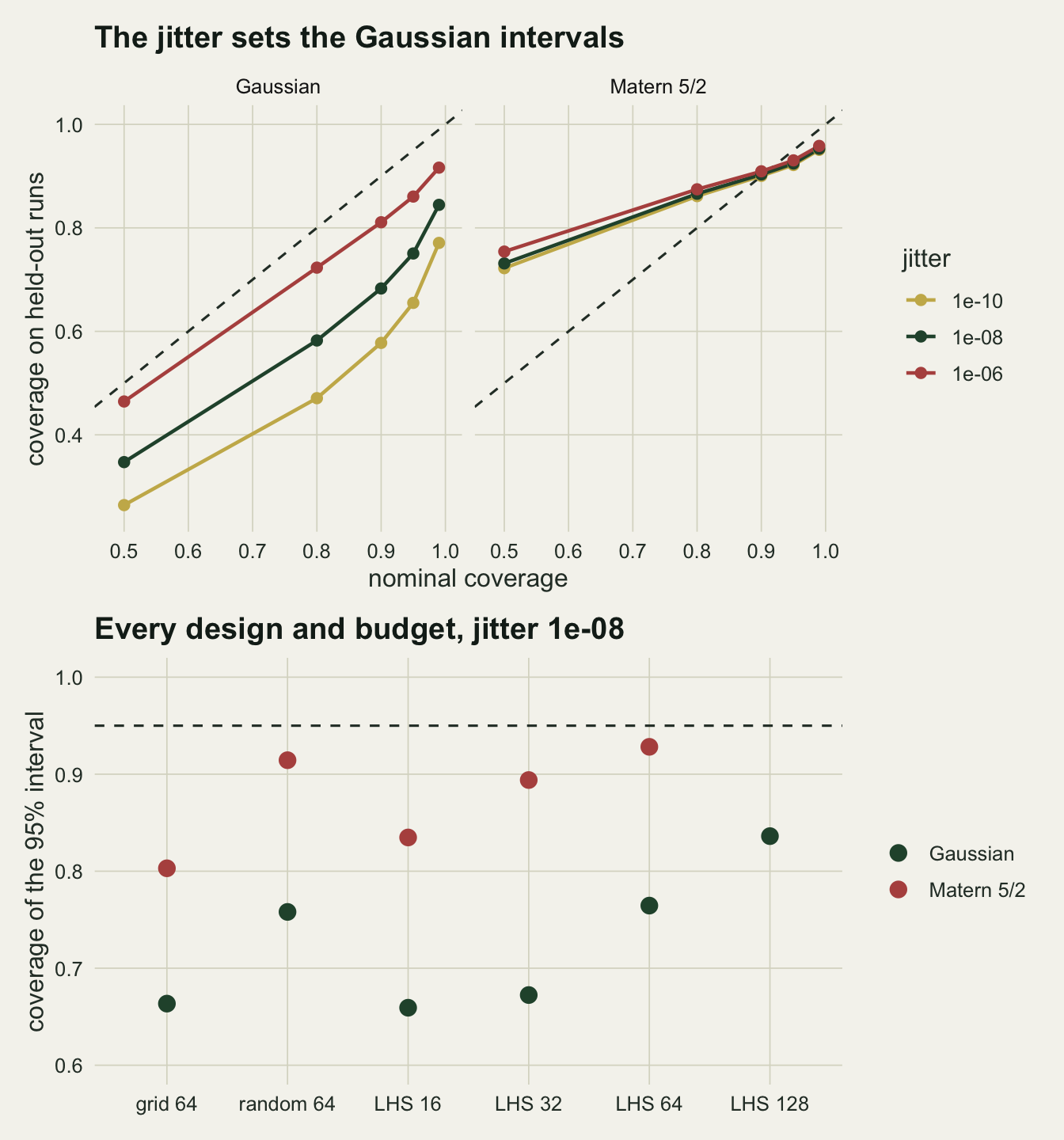
Across all forty sixty four run hypercubes the Matern intervals cover 92.8 per cent (Monte Carlo standard error 0.5 percentage points) against 76.5 per cent (standard error 1.3 points) for the Gaussian, and the standard deviation of their standardised errors is 1.08. They are not calibrated either. At the nominal fifty per cent level they cover 74.1 per cent, too wide in the middle, and at ninety nine per cent 95.6 per cent, slightly short in the tails. The grid and the small budgets fall short under both correlations: the Matern grid covers 80.3 per cent and sixteen hypercube runs 83.5 per cent. The Matern emulator was not fitted at one hundred and twenty eight runs, to keep the knit short.
Running the next simulation where the variance is largest
Ranking is enough for choosing where to run next. Start with a small Latin hypercube, fit, predict the standard deviation over a large set of candidate parameter combinations, run the simulator at the candidate with the largest one, and repeat. The runs go where the emulator is least sure. Here the start is sixteen runs, the candidates are two thousand fresh uniform points in each replicate, the length-scales are refitted after every eighth new run, and the procedure stops at sixty four so that it spends the same budget as the designs above. All of those constants were set before the first replicate.
n_seq_rep <- 10; n_seq_start <- 16; refit_every <- 8; n_cand <- 2000
set.seed(5528)
run_count <- 0
seq_example <- NULL
seq_tab <- do.call(rbind, lapply(seq_len(n_seq_rep), function(i) {
  X <- lhs_design(n_seq_start); y <- simulator(X)
  cand <- matrix(runif(n_cand * 3), ncol = 3)
  out <- NULL; par <- NULL
  while (nrow(X) <= n_design) {
    if ((nrow(X) - n_seq_start) %% refit_every == 0) {
      par <- fit_gp(X, y)$par
      p <- predict_gp(par, X, y, x_test)
      out <- rbind(out, data.frame(rep = i, runs = nrow(X), rmse = sqrt(mean((y_test - p$mu)^2))))
    }
    if (nrow(X) == n_design) break
    pc <- predict_gp(par, X, y, cand)
    pick <- which.max(pc$sd)
    X <- rbind(X, cand[pick, , drop = FALSE]); y <- c(y, simulator(cand[pick, , drop = FALSE]))
    cand <- cand[-pick, , drop = FALSE]
  }
  if (i == 1) seq_example <<- X
  out
}))
runs_seq <- run_count
seq_mean <- aggregate(rmse ~ runs, data = seq_tab, FUN = mean)
s_rmse <- function(nb) seq_mean$rmse[seq_mean$runs == nb]
s_mcse <- function(nb) sd(seq_tab$rmse[seq_tab$runs == nb]) / sqrt(n_seq_rep)
added <- seq_example[-seq_len(n_seq_start), ]
edge_share <- mean(apply(added, 1, function(p) any(p < 0.05 | p > 0.95)))
edge_share_unif <- 1 - 0.9^3   # uniform point within 0.05 of some face of the cube
seq_gain64 <- 1 - s_rmse(64) / b_rmse(64)
z_gain <- function(nb) (b_rmse(nb) - s_rmse(nb)) / sqrt(s_mcse(nb)^2 + b_sd(nb)^2 / sum(budget_tab$runs == nb))
z_gain64 <- z_gain(64); z_gain32 <- z_gain(32)
Over 10 replicates, which spent 640 runs in total, the sequential design reaches a test error of 0.0077 at thirty two runs (Monte Carlo standard error 0.0006) against 0.0090 for a one-shot hypercube of that size, and 0.0023 at sixty four (standard error 0.0002) against 0.0029. At the full budget that is 20 per cent less error for the same number of runs, a difference of 2.4 standard errors; at thirty two runs the difference is 1.6 standard errors. The gain is modest, and ten replicates measure it only coarsely.
Where the added runs went is the more instructive part. In the replicate drawn in the figure, 96 per cent of the forty eight added runs sit within a twentieth of the box of some face of the cube, where a uniformly scattered point would land there 27 per cent of the time. A stationary Gaussian process is least sure at the edges and corners, because a point there has neighbours on one side only, so maximum variance pushes the runs outward. On this simulator and a test set spread evenly over the box, that still paid. For a question that lives in the interior, such as the stock at the harvest rates actually being considered, the same rule would spend much of the budget where nobody is asking.
stage_lev <- c("first 16, Latin hypercube", "added at maximum variance")
seq_pts <- data.frame(r = seq_example[, 1], h = seq_example[, 2],
                      stage = factor(rep(stage_lev, c(n_seq_start, n_design - n_seq_start)),
                                     levels = stage_lev))
p_pts <- ggplot(seq_pts, aes(r, h, colour = stage)) +
  geom_point(size = 1.8) +
  scale_colour_manual(values = c(te_forest, te_rust), name = NULL) +
  coord_equal() +
  labs(x = "growth rate, scaled", y = "harvest rate, scaled", title = "Where the runs went") +
  theme_datasheet() + theme(legend.position = "bottom", legend.direction = "vertical")
curve_tab <- rbind(
  data.frame(method = "sequential, maximum variance", seq_mean),
  data.frame(method = "one-shot Latin hypercube",
             budget_mean[budget_mean$runs <= n_design, c("runs", "rmse")]))
p_curve <- ggplot(curve_tab, aes(runs, rmse, colour = method)) +
  geom_line(linewidth = 0.9) + geom_point(size = 2) +
  scale_y_log10() + scale_x_continuous(breaks = seq(16, 64, 16)) +
  scale_colour_manual(values = c(te_gold, te_rust), name = NULL) +
  labs(x = "simulator runs", y = "test RMSE", title = "Error against runs") +
  theme_datasheet() + theme(legend.position = "bottom", legend.direction = "vertical")
p_pts + p_curve + plot_annotation(theme = theme_datasheet())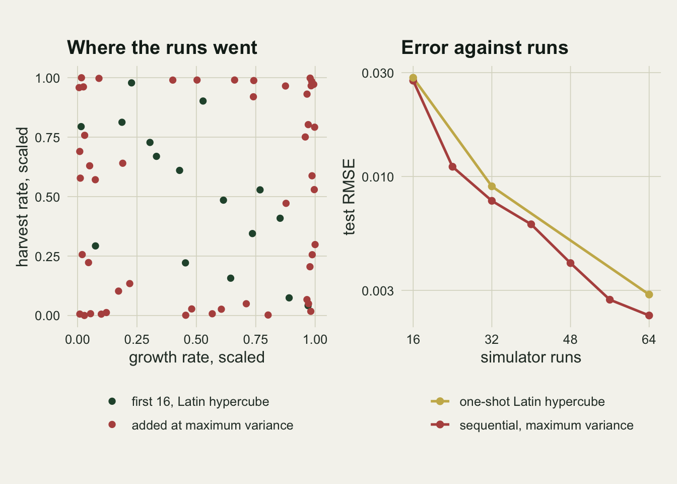
A box that crosses the collapse edge
Everything so far lives in a box where harvest is always below growth. Widen the box to growth rates from 0.1 to 1 and harvest rates from 0 to 0.4, and part of it now describes populations harvested faster than they can grow, which decline towards zero. The output is still a continuous function of the parameters, but it has a crease along the line where harvest equals growth: flat near zero on one side, rising on the other. The same machinery, the same test set positions and twenty Latin hypercubes of sixty four runs were used.
wide_lo <- c(r = 0.1, h = 0.0, theta = 0.5)
wide_hi <- c(r = 1.0, h = 0.4, theta = 3.0)
set.seed(6044)
run_count <- 0
y_test_wide <- simulator(x_test, wide_lo, wide_hi)
wide_nat <- to_natural(x_test, wide_lo, wide_hi)
collapse_share <- mean(wide_nat[, 2] > wide_nat[, 1])
near_edge <- abs(wide_nat[, 2] - wide_nat[, 1]) < 0.1
wide_scores <- t(replicate(20, {
  X <- lhs_design(n_design); y <- simulator(X, wide_lo, wide_hi)
  f <- fit_gp(X, y); p <- predict_gp(f$par, X, y, x_test)
  e <- y_test_wide - p$mu; z <- e / p$sd
  fm <- fit_gp(X, y, kernel = "matern"); pm <- predict_gp(fm$par, X, y, x_test, "matern")
  c(rmse = sqrt(mean(e^2)), rmse_near = sqrt(mean(e[near_edge]^2)),
    rmse_far = sqrt(mean(e[!near_edge]^2)), cover = mean(abs(z) < qnorm(0.975)),
    ell_r = exp(f$par[1]), ell_h = exp(f$par[2]), loo = loo_rmse(f$par, X, y),
    rmse_m = sqrt(mean((y_test_wide - pm$mu)^2)),
    cover_m = mean(abs(y_test_wide - pm$mu) < qnorm(0.975) * pm$sd))
}))
runs_wide <- run_count
wide_mean <- colMeans(wide_scores)
wide_sd <- sd(y_test_wide)
# length-scales in natural units: scaled length-scale times the width of that input's range
ell_nat_wide <- wide_mean[c("ell_r", "ell_h")] * (wide_hi - wide_lo)[1:2]
ell_nat_one <- ell_one[1:2] * (box_hi - box_lo)[1:2]
In the wide box 13.7 per cent of the test points lie beyond the collapse edge, and the output standard deviation grows to 0.326. The emulators average a test error of 0.0665, which is 20.4 per cent of that standard deviation, against 2.3 per cent in the persistent box for the same budget. For test points where harvest and growth differ by less than 0.1 the error is 0.0909; everywhere else it is 0.0583. The crease does not just spoil its own neighbourhood. A Gaussian correlation has one length-scale per input for the whole box, and with the crease inside the box those length-scales come out short (converted to natural units, because the two boxes have different widths, the mean fitted length-scales are 0.24 for growth and 0.18 for harvest, against 1.21 and 0.65 for the single emulator in the first box), and a short length-scale throws away information on the smooth side too. Nominal ninety five per cent intervals covered 80.0 per cent of held-out runs. Here the order of the two correlation functions reverses on error: a Matern 5/2 emulator on the same designs has an average test error of 0.0480, and its intervals cover 89.7 per cent.
The fit gives two warnings of its own. The length-scales are shorter, though a reader without the first box to compare against would have no reason to find them short. The leave-one-out error is 0.0554, which is 17.0 per cent of the output standard deviation (2.0 per cent in the first box). That warning does not need the first box: an emulator that misses its own left-out runs by a sixth of the output’s spread is visibly not a close stand-in for the simulator. The remedy has to come from outside the emulator: know where the simulator has thresholds, and consider emulating each regime separately with runs placed on both sides of the edge. That was not tried here.
What to report
Report the simulator runs by purpose: how many built the emulator, how many tested it, and how the design was drawn. For a Latin hypercube say whether it was a plain one or optimised for spacing, because the plain one controls one dimensional coverage only, and this post found it no better than random points for building an emulator.
Report the error of the emulator on runs it did not see, in the units of the output and as a fraction of the output’s standard deviation, and never the fit at the design points alone. If no runs can be spared for testing, report the leave-one-out error, which costs nothing: it flagged the grid in this post, which was 3.4 times less accurate than a hypercube of the same size, though it did not rank the hypercubes among themselves. A miss at the design runs larger than the held-out test error is a sign of a degenerate fit: the grid’s was, and none of the eighty hypercube and random fits did the same. A process variance above the output’s variance is not a warning on its own, because every one of those fits had one at least 8 times as large.
Report the estimated length-scales with the inputs they belong to, on the scaled box. They are the emulator’s summary of which inputs move the output over short distances, and a length-scale sitting on or near an optimiser bound is a problem that should be visible to a reader. Name the correlation function, and report the jitter or the estimated nugget with the lower bound of its search.
Report the held-out coverage of the emulator’s intervals beside the intervals, and refit at a second jitter to see whether it moves. Every Gaussian emulator here claimed ninety five per cent and, at the jitter used throughout, delivered between 66 and 84 per cent, a figure that belonged to the jitter as much as to the runs; the Matern emulators delivered between 80 and 93 per cent and, on the hypercubes where it was checked, hardly moved with the jitter. If the emulator’s uncertainty is carried into a decision, prefer a correlation whose coverage does not depend on the jitter, accept that in the smooth box it cost accuracy (the Matern test error was 1.34 times the Gaussian one on the same hypercubes), and still say how far short of nominal it was.
Honest limits
The simulator is a smooth three parameter differential equation with a scalar output. Real individual based models are stochastic, and their output at fixed parameters is a distribution, so a real emulator needs a nugget that is not jitter, replicate runs at some design points, and a decision about whether it is emulating the mean or the whole distribution. None of that was tested. The fact that the estimated nugget stayed at or below jitter size is a property of a deterministic simulator, not a general finding.
Three inputs is a small problem. The grid failed with four levels per input; in five inputs no grid with the same number of levels on every input has sixty four runs, and in ten dimensions the difference between a plain Latin hypercube and random points may well favour the hypercube again, as each axis becomes more sparsely covered. The finding that the two were indistinguishable is for this dimension and this budget. Spacing-optimised hypercubes, such as maximin designs, were not tried and are what the design literature would use.
Two correlation functions were compared, both with a constant mean. The jitter sweep used twenty hypercubes and three jitters, the Matern emulator was not fitted at one hundred and twenty eight runs, and the sequential design ranked its candidates by the Gaussian standard deviation at a single jitter; whether its choices move with the jitter was not checked. A Matern 3/2 correlation, or a linear mean in the inputs that would absorb some of the trend the process now carries, were not tried and could change both the errors and the coverage.
The test set is uniform over the box, so every error and coverage figure is an average over the box with equal weight everywhere. A manager who cares about a narrow band of harvest rates cares about the error there, which can be larger or smaller. The sequential design, in particular, was scored on a uniform test set while it put most of its runs on the faces of the box; scored on a test set concentrated in the interior it may compare less well, and that was not measured.
Integrating over the length-scales was measured on one design only, with a flat prior inside the optimiser bounds and a short Metropolis run, so its small gain is a measurement for that design rather than a general result; it says the length-scales were not the main cause here, and the jitter sweep and the Matern comparison say what was. Kennedy and O’Hagan’s framework goes further again, adding a discrepancy between the simulator and reality, and this post stops well short of calibrating anything against field data.
References
Sacks J, Welch WJ, Mitchell TJ, Wynn HP 1989 Statistical Science 4(4):409-423 (10.1214/ss/1177012413)
McKay MD, Beckman RJ, Conover WJ 1979 Technometrics 21(2):239-245 (10.1080/00401706.1979.10489755)
Kennedy MC, O’Hagan A 2001 Journal of the Royal Statistical Society Series B 63(3):425-464 (10.1111/1467-9868.00294)
Loeppky JL, Sacks J, Welch WJ 2009 Technometrics 51(4):366-376 (10.1198/TECH.2009.08040)