library(ggplot2)

te_pal <- list(forest = "#275139", green = "#2f8f63", sage = "#93a87f",
               clay = "#b5534e", gold = "#cda23f", line = "#dad9ca",
               ink = "#16241d", paper = "#f5f4ee")

theme_te <- function() {
  theme_minimal(base_size = 12) +
    theme(panel.grid.minor = element_blank(),
          panel.grid.major = element_line(colour = "#e7e6dc"),
          plot.background = element_rect(fill = "#f5f4ee", colour = NA),
          panel.background = element_rect(fill = "#f5f4ee", colour = NA),
          plot.title = element_text(face = "bold", colour = te_pal$ink),
          axis.title = element_text(colour = "#2c3a31"),
          axis.text = element_text(colour = "#2c3a31"),
          legend.position = "bottom")
}Checking an annual flux budget
R
eddy covariance
carbon flux
model checking
ecology tutorial
Six checks on a published eddy covariance carbon budget in R: friction velocity threshold spread, gap-filled half hours, and a defensible-choice multiverse.
A closed-path eddy covariance system sits at the top of a thirty metre mast in a temperate deciduous forest at forty-seven degrees north, with the canopy about ten metres below the sensor. It has been running for a year. The group that processed the record did what the community asks for: despiking, coordinate rotation, a friction velocity screen on the night-time data, a look-up table fill for everything the screen and the weather took out, and a sum over the year.
The paper reports one number and a standard error next to it. The site is a net carbon sink, the standard error is a few grams of carbon per square metre per year, and nothing in the manuscript suggests the sink is in doubt. That number then goes into a synthesis, and from there into a regional budget, and nobody who uses it will ever see the half hours it came from.
This post runs six checks on that finished budget. Each one asks a question that can be answered with a number, and each one comes back with a verdict on this particular study. They are: whether the friction velocity threshold was treated as a fixed quantity when it is not one, how much of the annual sum was measured rather than modelled, whether the gaps are in the half hours that carry the carbon, what the reported standard error actually contains, whether the sink claim survives the choices a different analyst would defensibly have made, and what the sign convention and the air below the sensor do to the total.
Three neighbouring posts hold the machinery this one leaves alone. Night-time flux and the u-star threshold is where the threshold comes from and how it is estimated; nothing here re-derives that estimator, and the only question asked about it is what happens to the year when its answer moves. Gap filling a flux time series sets out the filling methods and measures them against each other; here they are used exactly as they come, and the only question about them is how much of the annual total they carry. Partitioning net flux into GPP and respiration splits the measured flux into its two components; this post never splits anything, because the quantity under test is a net sum. The shape of the post follows checking a decomposition analysis, which does the same job for a litterbag study.
The year is simulated, for the reason that always applies to a checking post: a simulated tower year comes with a truth column, so each check ends in a verdict rather than an opinion. The parameters are ordinary ones for a mid-latitude broadleaf site, and the honest limits of running the checks against a known answer are set out near the end.
The study under test
The drivers come first, because everything else hangs off them. Photosynthetic photon flux density is a clear-sky curve for the latitude multiplied by a daily clearness index that carries over from one day to the next, air temperature is a seasonal cycle plus a persistent weather anomaly plus a diurnal swing that is wider on clear days, and canopy development is a pair of logistic curves that open the canopy in late April and close it in mid-October.
conv <- 1800 * 12.011e-6
n_day <- 365
per_day <- 48
n_hh <- n_day * per_day
doy <- rep(seq_len(n_day), each = per_day)
hod <- rep(seq(0, 23.5, by = 0.5), n_day)

lat_rad <- 47 * pi / 180
decl <- 23.44 * pi / 180 * sin(2 * pi * (doy - 81) / 365)
hr_ang <- (hod - 12) * 15 * pi / 180
sin_elev <- sin(lat_rad) * sin(decl) + cos(lat_rad) * cos(decl) * cos(hr_ang)
ppfd_pot <- 2100 * pmax(0, sin_elev)
night <- ppfd_pot < 5

set.seed(20260802)
kt_day <- numeric(n_day)
kt_day[1] <- 0.62
for (d in 2:n_day) {
  kt_day[d] <- 0.58 + 0.55 * (kt_day[d - 1] - 0.58) + rnorm(1, 0, 0.17)
}
kt_day <- pmin(0.95, pmax(0.16, kt_day))
ppfd <- ppfd_pot * pmin(1, rep(kt_day, each = per_day) * exp(rnorm(n_hh, 0, 0.12)))

wx <- numeric(n_day)
for (d in 2:n_day) wx[d] <- 0.75 * wx[d - 1] + rnorm(1, 0, 1.9)
tair <- 9 - 10 * cos(2 * pi * (doy - 15) / 365) + rep(wx, each = per_day) +
  (3.5 + 3 * rep(kt_day, each = per_day)) * sin(2 * pi * (hod - 9) / 24)
phen <- 1 / (1 + exp(-(doy - 118) / 7)) * 1 / (1 + exp((doy - 288) / 9))

print(round(c(half_hours = n_hh, night_share = mean(night),
              mean_air_temperature = mean(tair),
              warmest_half_hour = max(tair), coldest_half_hour = min(tair),
              midsummer_midday_ppfd = mean(ppfd[doy > 170 & doy < 200 &
                                                  hod > 11 & hod < 13]),
              days_with_full_canopy = sum(phen > 0.9) / per_day), 3))
half_hours night_share mean_air_temperature
17520.000 0.501 8.201
warmest_half_hour coldest_half_hour midsummer_midday_ppfd
28.240 -15.793 1079.402
days_with_full_canopy
135.000 That is 17520 half hours, 50.1 per cent of them at night, with a mean air temperature of 8.20 degrees C and 135 days of full canopy. Midday photon flux density in midsummer averages 1079 umol/m2/s once cloud is taken off the clear-sky value.
Now the ecosystem and the instrument. Gross uptake is a rectangular hyperbola in light scaled by canopy development, respiration is an exponential in temperature with a smaller base outside the growing season, and net exchange is respiration minus uptake, positive towards the atmosphere.
The instrument adds three things. The first is the failure that gives this post its subject: on calm nights the eddy flux under-measures respiration, because the carbon respired by soil and stems does not reach the sensor as turbulence. The attenuation is written here as the ratio of friction velocity to a site threshold, capped at one, which is the standard idealisation. What that threshold is worth is the whole of check 1, so the simulation makes it deliberately awkward: the true threshold is higher under a full canopy than a bare one, and it varies from night to night with stability and wind direction. The second is heteroscedastic noise with a double exponential shape, which is what Richardson and Hollinger (2007) and the paired-tower literature report for half-hourly flux errors. The third is downtime: calibration blocks, power cuts and rain rejection.
set.seed(20260803)
alpha <- 0.055
amax <- 30
r10 <- 3.9
q10 <- 2.0
gpp <- phen * alpha * ppfd * amax / (alpha * ppfd + amax)
reco <- (0.35 + 0.65 * phen) * r10 * q10^((tair - 10) / 10)
flux_true <- reco - gpp
truth <- sum(flux_true) * conv

u_scale <- exp(rnorm(n_day, 0, 0.24))
u_true <- (0.14 + 0.14 * phen) * rep(u_scale, each = per_day)
ustar <- rep(exp(rnorm(n_day, log(0.36), 0.42)), each = per_day) *
  exp(rnorm(n_hh, 0, 0.33)) * ifelse(night, 0.60, 1.30)
att <- pmin(1, ustar / u_true)
flux_att <- ifelse(night, flux_true * att, flux_true)

sd_hh <- 0.60 + 0.30 * abs(flux_att)
lap <- sd_hh / sqrt(2) * (rexp(n_hh) - rexp(n_hh))
nee_raw <- flux_att + lap

gone <- rep(FALSE, n_hh)
for (b in seq_len(20)) {
  s0 <- sample.int(n_hh - 100, 1)
  gone[s0:(s0 + sample(12:96, 1))] <- TRUE
}
gone <- gone | (runif(n_hh) < ifelse(night, 0.085, 0.045) +
                  ifelse(ppfd < 0.30 * ppfd_pot, 0.18, 0))
nee_obs <- ifelse(gone, NA_real_, nee_raw)

print(round(c(annual_gpp = sum(gpp) * conv,
              annual_respiration = sum(reco) * conv,
              true_annual_nee = truth,
              median_threshold_leafless = median(u_true[phen < 0.05]),
              median_threshold_full_canopy = median(u_true[phen > 0.95]),
              threshold_5th = unname(quantile(u_true, 0.05)),
              threshold_95th = unname(quantile(u_true, 0.95)),
              night_half_hours_below_their_threshold =
                mean(ustar[night] < u_true[night]),
              downtime_share = mean(gone)), 4))
annual_gpp annual_respiration
1487.4325 1221.6913
true_annual_nee median_threshold_leafless
-265.7412 0.1439
median_threshold_full_canopy threshold_5th
0.2780 0.1131
threshold_95th night_half_hours_below_their_threshold
0.3729 0.4082
downtime_share
0.1322 The year the tower is standing over takes up 1487.4 gC/m2 and respires 1221.7 gC/m2, for a true net exchange of -265.7 gC/m2/yr. That is the number every check below is scored against, and it is a sink of unremarkable size for a mid-latitude broadleaf forest.
The threshold in the generator has a median of 0.144 m/s when the canopy is bare and 0.278 m/s when it is full, with a fifth to ninety-fifth percentile range across the year of 0.113 to 0.373 m/s. 40.8 per cent of night half hours fall below whatever their own threshold happened to be that night, and 13.2 per cent of the year is lost to downtime before any screening is applied. Aubinet (2008) is the standard account of why the night-time flux behaves this way and of how much of it the friction velocity criterion can and cannot repair.
The pipeline below is the analyst’s, not the ecosystem’s. A binned threshold estimator of the usual kind is applied to the screened night data, the screen is applied at whatever it returns, and the gaps are filled from a look-up table of measured half hours in the same fortnight, the same half of the day and the same radiation or temperature class. Papale et al (2006) is the reference implementation of that sequence and the reason it is close to universal.
est_thr <- function(uu, ff, tt) {
  ok <- !is.na(ff)
  uu <- uu[ok]; ff <- ff[ok]; tt <- tt[ok]
  if (length(ff) < 400) return(NA_real_)
  tb <- cut(tt, unique(quantile(tt, seq(0, 1, length.out = 7))),
            include.lowest = TRUE)
  got <- numeric(0)
  for (lv in levels(tb)) {
    k <- which(tb == lv)
    if (length(k) < 120) next
    ub <- cut(uu[k], unique(quantile(uu[k], seq(0, 1, length.out = 21))),
              include.lowest = TRUE)
    mb <- tapply(ff[k], ub, mean)
    um <- tapply(uu[k], ub, mean)
    j_ok <- which(!is.na(mb))
    for (j in j_ok) {
      hi <- j_ok[j_ok > j]
      if (length(hi) < 3) break
      if (mb[j] >= 0.95 * mean(mb[hi])) { got <- c(got, um[j]); break }
    }
  }
  if (!length(got)) NA_real_ else median(got)
}

win <- pmin(26, ((doy - 1) %/% 14) + 1)
rad_cls <- cut(ppfd, c(-1, 5, 200, 500, 900, 1400, Inf), labels = FALSE)
tmp_cls <- cut(tair, c(-Inf, 0, 5, 10, 15, 20, Inf), labels = FALSE)
cell_a <- paste(win, ifelse(night, paste0("n", tmp_cls), paste0("d", rad_cls)))
cell_b <- paste(ifelse(night, "n", "d"), ifelse(night, tmp_cls, rad_cls))

lut_pred <- function(y) {
  m1 <- tapply(y, cell_a, mean, na.rm = TRUE)
  m2 <- tapply(y, cell_b, mean, na.rm = TRUE)
  v1 <- as.numeric(m1[cell_a])
  v2 <- as.numeric(m2[cell_b])
  v1[is.na(v1)] <- v2[is.na(v1)]
  v1
}
apply_fill <- function(y, f) {
  v <- f(y)
  out <- y
  idx <- is.na(y)
  out[idx] <- v[idx]
  gl <- tapply(y, night, mean, na.rm = TRUE)
  bad <- is.na(out)
  out[bad] <- as.numeric(gl[as.character(night[bad])])
  out
}
screen_at <- function(thr) ifelse(!gone & !(night & ustar < thr), nee_raw, NA_real_)
bud_at <- function(thr, f) sum(apply_fill(screen_at(thr), f)) * conv

nt <- night & !is.na(nee_obs)
thr_hat <- est_thr(ustar[nt], nee_obs[nt], tair[nt])
y_ana <- screen_at(thr_hat)
fil_ana <- apply_fill(y_ana, lut_pred)
rep_bud <- sum(fil_ana) * conv
is_fill <- is.na(y_ana)
obs_i <- which(!is_fill)

cm <- lut_pred(y_ana)
res_o <- (y_ana - cm)[obs_i]
mag_o <- abs(cm)[obs_i]
mb_o <- cut(mag_o, quantile(mag_o, seq(0, 1, length.out = 13)),
            include.lowest = TRUE)
sc <- data.frame(m = as.numeric(tapply(mag_o, mb_o, mean)),
                 s = as.numeric(tapply(res_o, mb_o, sd)))
sig_fit <- lm(s ~ m, data = sc)
sig_i <- pmax(0.2, predict(sig_fit, newdata = data.frame(m = abs(fil_ana))))
se_rand <- sqrt(sum(sig_i[obs_i]^2)) * conv

print(round(c(estimated_threshold = thr_hat,
              coverage_after_screening = 1 - mean(is_fill),
              reported_budget = rep_bud, reported_standard_error = se_rand,
              true_budget = truth, error = rep_bud - truth,
              error_in_reported_standard_errors = (rep_bud - truth) / se_rand), 4))
estimated_threshold coverage_after_screening
0.1709 0.7223
reported_budget reported_standard_error
-319.5117 6.1477
true_budget error
-265.7412 -53.7705
error_in_reported_standard_errors
-8.7465 print(round(c(error_sd_intercept = unname(coef(sig_fit)[1]),
error_sd_slope = unname(coef(sig_fit)[2])), 4))error_sd_intercept error_sd_slope
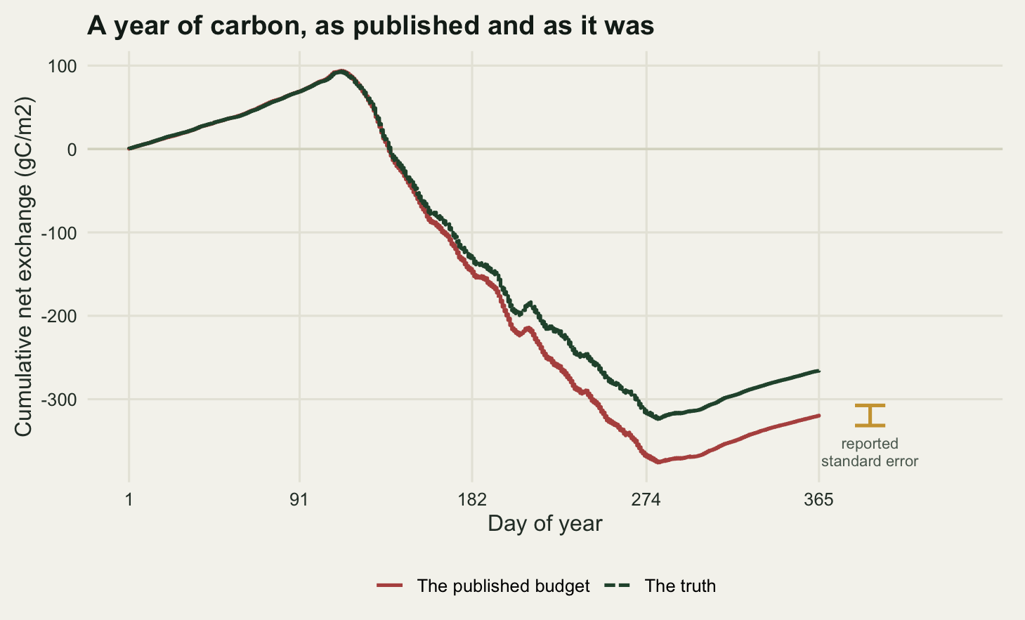
0.9717 0.3045 The estimator returns 0.1709 m/s, which leaves 72.2 per cent of the year as measured data, and the annual sum comes out at -319.5 gC/m2/yr.
The standard error next to it is the random measurement error propagated over the year. The scatter of measured half hours about their look-up cell means is binned by flux magnitude, a straight line is fitted through those bin standard deviations, giving an error standard deviation of 0.972 plus 0.304 times the flux, and the resulting variances are added in quadrature over the measured half hours. That gives 6.15 gC/m2/yr. It is small because independence across half hours is assumed, which is the assumption that Moncrieff, Malhi and Leuning (1996) set out for exactly this calculation, and which nothing in a published figure ever flags.
So the study under test says: a net sink of 319.5 gC/m2/yr, plus or minus 6.15. The truth is -265.7. The error is -53.8 gC/m2/yr, or 8.75 reported standard errors, and the sink is overstated by 20.2 per cent.
Check 1: was the threshold a number or a choice
The pipeline used one friction velocity threshold for the whole year and then forgot it. Everything downstream, the screen, the fill, the sum and the standard error, is conditional on that value being correct, and none of the uncertainty in it appears anywhere in the output.
The check resamples whole nights with replacement, re-estimates the threshold on each resample, and runs each of those thresholds through the entire pipeline to the annual sum. Whole nights rather than half hours, because the half hours inside a night share their stability, their wind direction and their footprint. This is the procedure Barr et al (2013) formalised for flux networks; the point here is not the estimator but what its spread is worth in grams of carbon.
set.seed(20260804)
n_boot <- 200
night_id <- ((seq_len(n_hh) - 1 + 24) %/% 48) + 1
nd <- sort(unique(night_id[night]))
by_night <- split(which(nt), night_id[nt])
thr_b <- numeric(n_boot)
for (b in seq_len(n_boot)) {
  idx <- unlist(by_night[as.character(sample(nd, length(nd), replace = TRUE))],
                use.names = FALSE)
  thr_b[b] <- est_thr(ustar[idx], nee_obs[idx], tair[idx])
}
bud_b <- vapply(thr_b, bud_at, numeric(1), f = lut_pred)
thr_ci <- quantile(thr_b, c(0.025, 0.975))
bud_ci <- quantile(bud_b, c(0.025, 0.975))
se_thr <- sd(bud_b)

grid_thr <- seq(0.05, 0.45, by = 0.0125)
sweep_thr <- t(vapply(grid_thr, function(th) {
  yy <- screen_at(th)
  c(threshold = th, filled = mean(is.na(yy)),
    budget = sum(apply_fill(yy, lut_pred)) * conv)
}, numeric(3)))
rownames(sweep_thr) <- sprintf("%.4f", grid_thr)

print(round(c(bootstrap_replicates = n_boot, nights_resampled = length(nd),
              threshold_lower = thr_ci[[1]], threshold_median = median(thr_b),
              threshold_upper = thr_ci[[2]]), 4))
bootstrap_replicates nights_resampled threshold_lower
200.0000 366.0000 0.1340
threshold_median threshold_upper
0.1780 0.2232 print(round(c(budget_lower = bud_ci[[1]], budget_upper = bud_ci[[2]],
threshold_interval_width = bud_ci[[2]] - bud_ci[[1]],
reported_interval_width = 2 * qnorm(0.975) * se_rand,
width_ratio = (bud_ci[[2]] - bud_ci[[1]]) /
(2 * qnorm(0.975) * se_rand),
sd_from_threshold = se_thr,
sd_reported = se_rand), 4)) budget_lower budget_upper threshold_interval_width
-342.4421 -295.4383 47.0038
reported_interval_width width_ratio sd_from_threshold
24.0984 1.9505 11.3378
sd_reported
6.1477 print(round(sweep_thr[seq(1, nrow(sweep_thr), by = 4), ], 4)) threshold filled budget
0.0500 0.05 0.1331 -371.0187
0.1000 0.10 0.1650 -358.1717
0.1500 0.15 0.2409 -333.5600
0.2000 0.20 0.3252 -306.4898
0.2500 0.25 0.3975 -289.5415
0.3000 0.30 0.4491 -284.8541
0.3500 0.35 0.4822 -278.1478
0.4000 0.40 0.5082 -273.6504
0.4500 0.45 0.5258 -273.7074Over 200 resamples of the 366 nights, the estimated threshold runs from 0.1340 to 0.2232 m/s, with a median of 0.1780. Put each of those through the pipeline and the annual budget runs from -342.4 to -295.4 gC/m2/yr.
That interval is 47.0 gC/m2/yr wide. The interval the paper printed, two standard errors either side of the estimate, is 24.1 wide. The ratio is 1.95. On standard deviations rather than intervals, the threshold contributes 11.34 gC/m2/yr against the reported 6.15, so it is the larger of the two by a factor of 1.84 and the reported figure omits 77.3 per cent of the variance those two sources produce between them.
The sweep says why. Screening at 0.05 m/s, which keeps almost every night half hour, gives -371.0 gC/m2/yr. Screening at 0.25 gives -289.5, and by 0.40 the curve has flattened at -273.7. Below the true range the budget is a steep function of the choice; above it the choice stops mattering, because everything that could be contaminated has already gone. The published threshold of 0.1709 sits on the steep part.
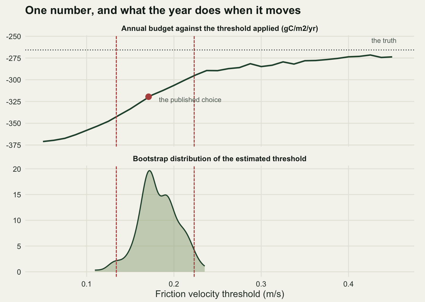
The verdict on this study is that the threshold is the dominant term in a budget that reports no term for it at all, and that the published interval is about half the width of the one the threshold alone requires. The deeper problem is visible in the generator: there is no single correct threshold to find, because the true one moves with the canopy and with the night. A bootstrap measures how well one number can be pinned down. It does not measure the cost of there being one number.
Check 2: how much of the year was measured
The annual sum is a sum over every half hour in the year, and only some of those half hours are measurements. The rest are outputs of the fill. The share of half hours that were filled is the figure that gets reported when anything is reported; the share of the carbon that came from filled half hours is a different figure, and the difference between them is the check.
c_fill <- sum(fil_ana[is_fill]) * conv
c_meas <- sum(fil_ana[obs_i]) * conv
share_gross <- sum(abs(fil_ana[is_fill])) / sum(abs(fil_ana))

print(round(c(share_of_half_hours_filled = mean(is_fill),
              carbon_from_filled_half_hours = c_fill,
              carbon_from_measured_half_hours = c_meas,
              filled_over_the_reported_budget = abs(c_fill / rep_bud),
              filled_share_of_gross_exchange = share_gross,
              night_total = sum(fil_ana[night]) * conv,
              night_total_from_filled = sum(fil_ana[night & is_fill]) * conv,
              filled_share_of_night_half_hours = mean(is_fill[night]),
              filled_share_of_night_carbon =
                sum(fil_ana[night & is_fill]) / sum(fil_ana[night])), 4))
share_of_half_hours_filled carbon_from_filled_half_hours
0.2777 93.2399
carbon_from_measured_half_hours filled_over_the_reported_budget
-412.7516 0.2918
filled_share_of_gross_exchange night_total
0.2003 384.8927
night_total_from_filled filled_share_of_night_half_hours
165.7024 0.4320
filled_share_of_night_carbon
0.4305 27.8 per cent of the half hours in the year were filled. Those half hours contribute 93.2 gC/m2 to the annual total, against -412.8 gC/m2 from the measured ones. As a share of the gross exchange, the sum of the absolute contributions, the filled block is 20.0 per cent. As a share of the reported net budget it is 29.2 per cent.
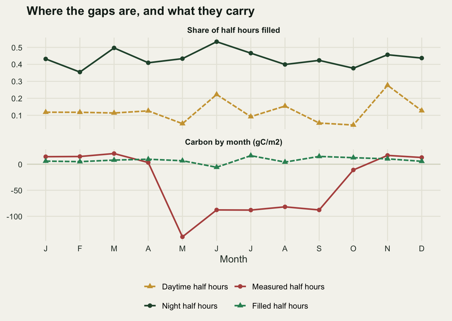
Three numbers, all correct, all describing the same block of the record, and they differ because the filled half hours are not a random sample of the year. About four in five of them are night half hours, where the flux is small and always the same sign, so they are under-represented in the gross exchange, which the large daytime fluxes dominate, and over-represented in the net total, which is a small difference between two large opposing sums. Take the filled block out of the year and the remaining measured half hours give -412.8 gC/m2, a sink 29.2 per cent larger than the one published.
Within the night alone the two figures come back together: 43.2 per cent of night half hours are filled and they carry 43.1 per cent of the night-time carbon. That is the useful diagnostic. When the filled share of half hours and the filled share of carbon match inside a stratum, the fill is doing an average job on an average subset of that stratum; when they diverge across the record as a whole, the divergence is telling you where the gaps are, not how good the fill is. Falge et al (2001) made the same distinction when the community first agreed what a defensible annual sum required.
Check 3: are the gaps where the carbon is
Check 2 said the gaps are concentrated somewhere. This one says where, and then asks what the budget would have been if the analyst had treated them as missing at random, which is what any procedure that scales up a mean of the measurements silently assumes.
seas_nm <- c("winter", "spring", "summer", "autumn",
             "winter")[cut(doy, c(0, 59, 151, 243, 334, 366), labels = FALSE)]
miss_tab <- tapply(is_fill,
                   list(factor(seas_nm, c("winter", "spring", "summer",
                                          "autumn")),
                        ifelse(night, "night", "day")), mean)
mcar <- mean(fil_ana[obs_i]) * n_hh * conv

print(round(miss_tab, 4))
day night
winter 0.1210 0.4112
spring 0.0941 0.4503
summer 0.1561 0.4618
autumn 0.1130 0.4198print(round(c(worst_day = max(miss_tab[, "day"]),
worst_night = max(miss_tab[, "night"]),
night_over_day = mean(miss_tab[, "night"]) /
mean(miss_tab[, "day"])), 4)) worst_day worst_night night_over_day
0.1561 0.4618 3.5999 print(round(c(budget_if_gaps_were_random = mcar,
reported_budget = rep_bud, true_budget = truth,
random_gaps_over_truth = mcar / truth,
random_gaps_minus_reported = mcar - rep_bud), 4))budget_if_gaps_were_random reported_budget
-571.4270 -319.5117
true_budget random_gaps_over_truth
-265.7412 2.1503
random_gaps_minus_reported
-251.9153 The table is the check. Daytime gaps run from 9.4 to 15.6 per cent across the four seasons; night-time gaps run from 41.1 to 46.2 per cent. On average the night is missing 3.60 times as often as the day, and this is not an accident of weather: the friction velocity screen is defined to remove night data and only night data, so a record processed this way is night-biased by construction.
Now the counterfactual. Suppose the gaps had been treated as missing at random, so that the mean of the measured half hours was scaled up to the length of the year. That gives -571.4 gC/m2/yr, against a truth of -265.7: a sink 2.15 times too large, and 251.9 gC/m2/yr away from the figure the group actually published.
The verdict on the reported sink is therefore mixed, and it should be stated in that order. The missingness is severely non-random, so any procedure that ignores the structure is off by more than two hundred grams. The look-up table fill does not ignore the structure, and that is the whole of what it buys: it does not make the night data appear, it only stops the day data standing in for it. The fill is not the weak point of this analysis. The threshold that decided which night half hours became gaps is.
Check 4: what the reported standard error contains
Three things can move the annual sum without anybody making a mistake. The measurements carry random error. The gaps have to be filled with something. And the threshold had to be chosen. The reported standard error covers the first of those. This check puts a number on all three and compares their sizes.
The random term is the one already computed: the fitted error standard deviation added in quadrature over the measured half hours. The filling term is the same operation over the filled half hours, using the scatter of measured values within each look-up cell, which is what is not known about a half hour that was replaced by its cell mean. The threshold term is the spread of the annual sum over the bootstrap in check 1.
There is one thing the filling term as written assumes, and the second block below tests it: that the cell means are unbiased. Two thousand measured half hours are hidden at a time, refilled by the same procedure, and the mean error of the fill on those artificial gaps is scaled up to the real gap count. Richardson and Hollinger (2007) built this into a method for the extra uncertainty that long gaps add, which is the part an artificial-gap study of scattered half hours will always miss.
cell_sd <- tapply(res_o, cell_a[obs_i], sd)
s_cell <- as.numeric(cell_sd[cell_a])
s_cell[is.na(s_cell)] <- mean(cell_sd, na.rm = TRUE)
se_fill <- sqrt(sum(s_cell[is_fill]^2)) * conv
se_tot <- sqrt(se_rand^2 + se_fill^2 + se_thr^2)

set.seed(20260805)
n_art <- 40
art <- numeric(n_art)
for (b in seq_len(n_art)) {
  pick <- sample(obs_i, 2000)
  yb <- y_ana
  yb[pick] <- NA
  art[b] <- mean(apply_fill(yb, lut_pred)[pick] - y_ana[pick])
}

print(round(c(random_measurement_error = se_rand, gap_filling = se_fill,
              threshold_choice = se_thr, quadrature_total = se_tot,
              reported_share_of_the_total_variance = se_rand^2 / se_tot^2,
              actual_error = rep_bud - truth,
              actual_error_in_total_sds = (rep_bud - truth) / se_tot), 4))
random_measurement_error gap_filling
6.1477 2.7570
threshold_choice quadrature_total
11.3378 13.1887
reported_share_of_the_total_variance actual_error
0.2173 -53.7705
actual_error_in_total_sds
-4.0770 print(round(c(artificial_gap_replicates = n_art,
fill_bias_per_half_hour = mean(art),
fill_bias_over_the_year = mean(art) * sum(is_fill) * conv,
monte_carlo_error_of_that =
sd(art) / sqrt(n_art) * sum(is_fill) * conv), 5))artificial_gap_replicates fill_bias_per_half_hour fill_bias_over_the_year
40.00000 0.01070 1.12508
monte_carlo_error_of_that
1.06007 The three contributions are 6.15 gC/m2/yr for random measurement error, 2.76 for filling and 11.34 for the threshold. The threshold dominates. It is 1.84 times the random term and 4.11 times the filling term, and in quadrature the three give 13.19 gC/m2/yr, of which the reported standard error is 21.7 per cent of the variance.
The filling term is the smallest of the three, which is not the ordering most people expect from a record with 27.8 per cent of its half hours modelled. The reason is arithmetic rather than skill: filling error accumulates like a random walk over 4865 half hours while the threshold moves all of them together. Choosing badly once is worth more than guessing imprecisely thousands of times.
The artificial gaps say the fill is close to unbiased on gaps of this kind. Over 40 replicates the mean fill error is 0.0107 umol/m2/s per half hour, which scaled to the real gap count is 1.13 gC/m2/yr with a Monte Carlo error of 1.06. That is indistinguishable from zero, and it should be read narrowly: it says the look-up table is not systematically wrong about the half hours it was given, not that the half hours it was given were the right ones.
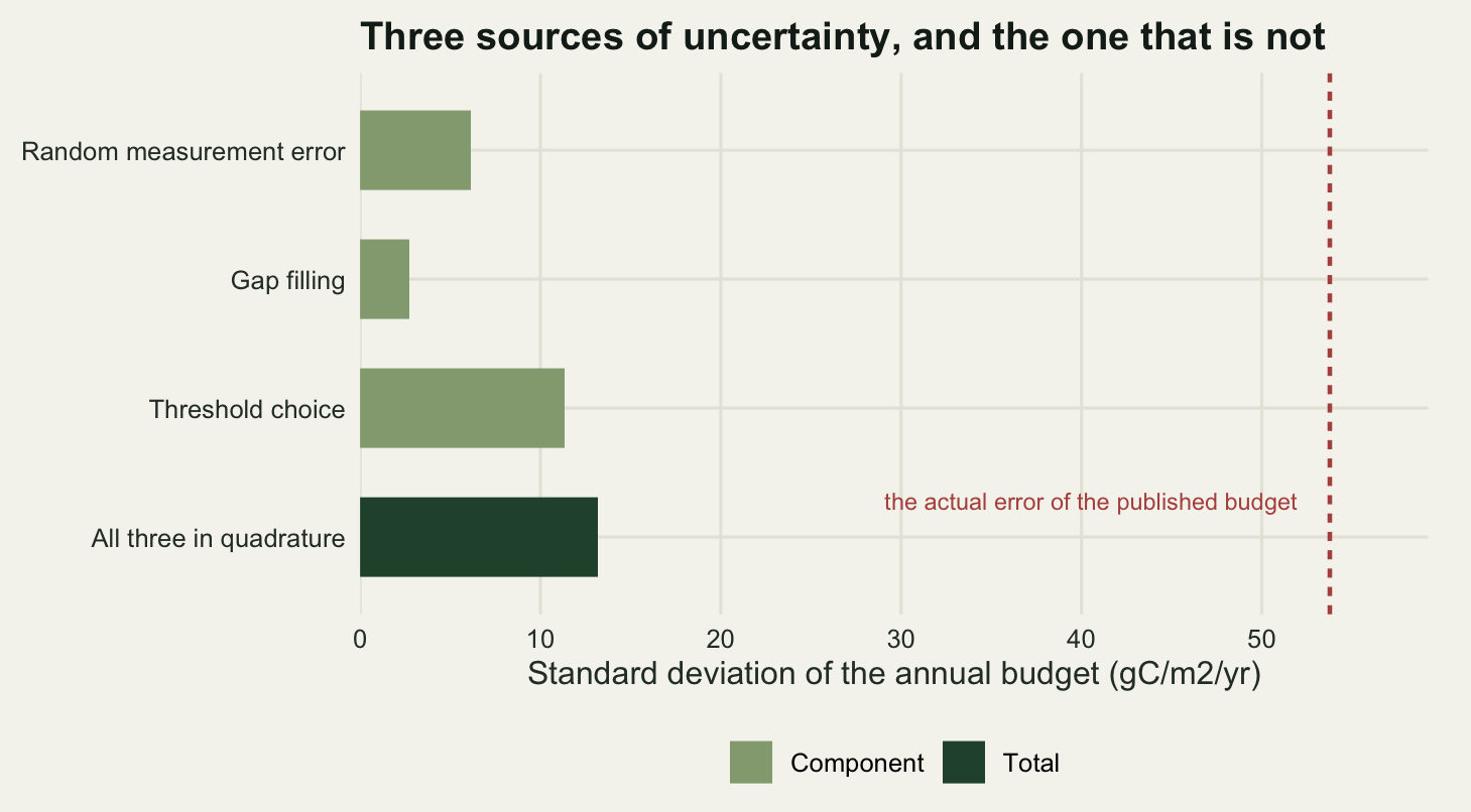
The last line of that table is the one to sit with. The actual error of the published budget is -53.8 gC/m2/yr, which is 4.08 times the combined standard deviation of all three terms. Widening the interval to include everything in this check would still not have covered the truth, because the error is not a draw from any of these distributions. It is a bias: the threshold estimate landed below the range the site actually needed, and attenuation is capped at one, so on the night half hours it let through it can only remove respiration, never add it. Every error it makes runs the same way, and the sink comes out too big.
Check 5: does the sink survive the defensible choices
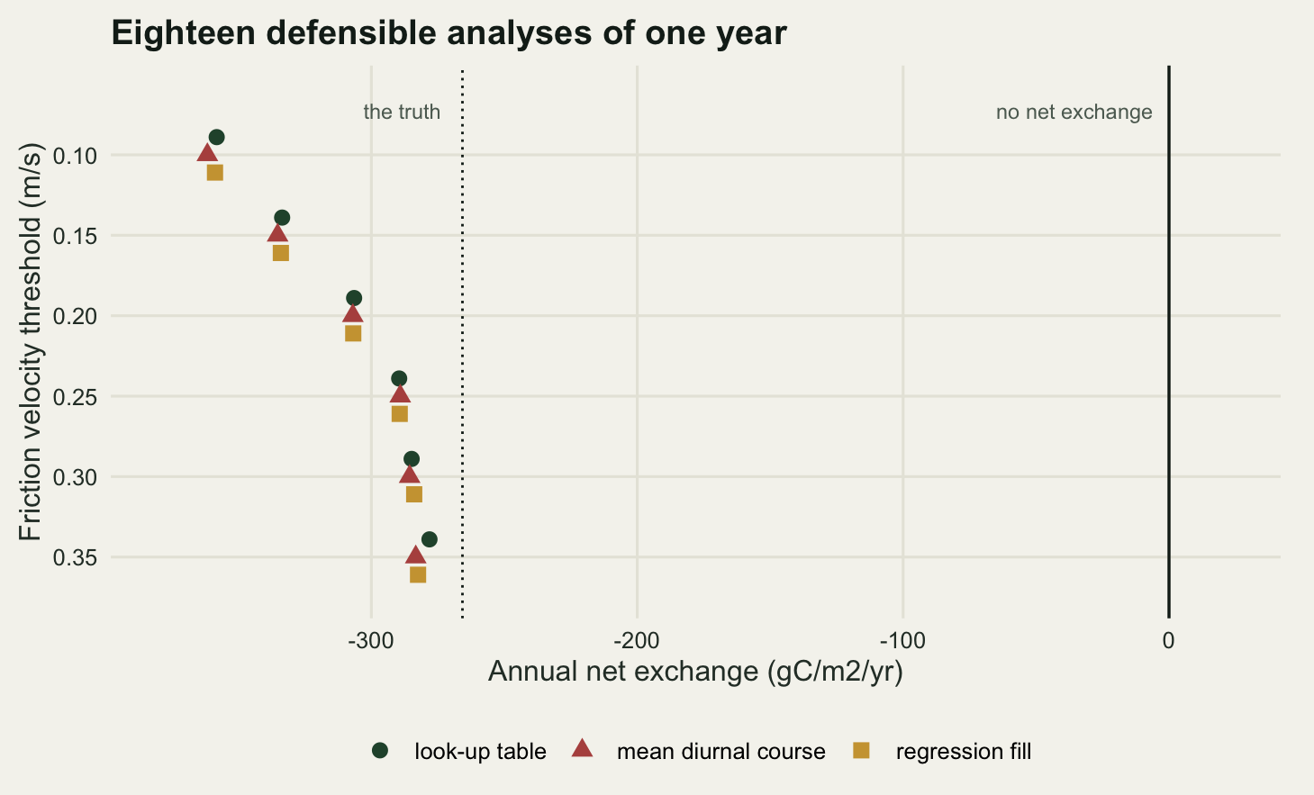
The multiverse is the cheapest check in the post and the one that travels best, because it needs no truth column and can be run on somebody else’s data. Take the choices that a competent second analyst might have made differently, cross them, compute the answer under each, and look at the spread. Here that is six friction velocity thresholds spanning the range that turns up in the forest literature, crossed with three ways of filling the gaps: the look-up table already in use, a mean diurnal course over a fifteen-day window at the same half hour, and a regression on radiation and temperature fitted in monthly windows.
mdv_pred <- function(y) {
  mm <- matrix(y, nrow = per_day)
  num <- mm
  num[is.na(num)] <- 0
  den <- !is.na(mm)
  acc_n <- matrix(0, per_day, n_day)
  acc_d <- matrix(0, per_day, n_day)
  for (k in -7:7) {
    j <- pmin(n_day, pmax(1, seq_len(n_day) + k))
    acc_n <- acc_n + num[, j, drop = FALSE]
    acc_d <- acc_d + den[, j, drop = FALSE]
  }
  out <- acc_n / pmax(1, acc_d)
  out[acc_d == 0] <- NA
  as.numeric(out)
}
reg_pred <- function(y) {
  w30 <- pmin(12, ((doy - 1) %/% 31) + 1)
  pred <- rep(NA_real_, n_hh)
  for (w in unique(w30)) {
    for (isn in c(TRUE, FALSE)) {
      k <- which(w30 == w & night == isn)
      if (sum(!is.na(y[k])) < 30) next
      dd <- data.frame(y = y[k], p = ppfd[k], tt = tair[k])
      mf <- if (isn) lm(y ~ tt + I(tt^2), data = dd)
            else lm(y ~ p + I(p^2) + tt, data = dd)
      pred[k] <- predict(mf, newdata = dd)
    }
  }
  pred
}

thr_set <- c(0.10, 0.15, 0.20, 0.25, 0.30, 0.35)
fills <- list(`look-up table` = lut_pred, `mean diurnal course` = mdv_pred,
              `regression fill` = reg_pred)
multi <- do.call(rbind, lapply(names(fills), function(nm) {
  data.frame(threshold = thr_set, method = nm,
             budget = vapply(thr_set, bud_at, numeric(1), f = fills[[nm]]))
}))

print(round(xtabs(budget ~ threshold + method, multi), 3))
method
threshold look-up table mean diurnal course regression fill
0.1 -358.172 -361.679 -358.810
0.15 -333.560 -335.265 -334.040
0.2 -306.490 -306.969 -306.815
0.25 -289.541 -289.137 -289.342
0.3 -284.854 -285.611 -283.890
0.35 -278.148 -283.308 -282.442print(round(c(combinations = nrow(multi),
still_a_sink = sum(multi$budget < 0),
largest_sink = min(multi$budget),
smallest_sink = max(multi$budget),
range_width = diff(range(multi$budget)),
range_in_reported_standard_errors =
diff(range(multi$budget)) / se_rand,
spread_across_fills_at_one_threshold =
diff(range(multi$budget[multi$threshold == 0.20])),
true_budget = truth), 4)) combinations still_a_sink
18.0000 18.0000
largest_sink smallest_sink
-361.6789 -278.1478
range_width range_in_reported_standard_errors
83.5311 13.5874
spread_across_fills_at_one_threshold true_budget
0.4791 -265.7412 All 18 analyses give a sink. Not most of them, all of them: the smallest is -278.1 gC/m2/yr and the largest is -361.7, and zero is nowhere near either end. That is a check that passed, and it should be reported as a result rather than skipped over. The claim in the paper, that this site took up carbon over the year, is not sensitive to any choice tested here.
The magnitude is another matter. The range across the multiverse is 83.5 gC/m2/yr, which is 13.6 times the reported standard error and 31.4 per cent of the true budget. A synthesis that treats the published value as 319.5 plus or minus 6.15 is combining a number that a defensible reanalysis could have moved by 84 grams.
Where that range comes from is the useful part. Fix the threshold at 0.20 and swap the fill through all three methods and the annual sum moves by 0.48 gC/m2/yr; the table has the fills further apart at the two ends of the threshold range, but never by more than a few grams. Fix the fill and move the threshold across its range and the sum moves by tens of grams. This matches what Moffat et al (2007) found when they compared filling techniques on real records: the annual sums from reasonable methods agree far more closely than anyone expects, and the effort is better spent elsewhere. On this record, elsewhere means the threshold.
Check 6: the sign convention, and the air under the sensor
Two short items that belong on any checklist for a published budget.
The first takes a second. A flux written positive towards the atmosphere and a flux written positive towards the ecosystem are the same measurement with opposite signs, and a budget that changes hands between a tower group, a modeller and a synthesis has several chances to be flipped. The cost is not subtle: for this study it is twice the budget, which is 639.0 gC/m2/yr, turning a moderate sink into a moderate source of the same size. The check is to state the convention next to the number, every time, and to sanity-check the sign of the night-time mean, which must be positive towards the atmosphere in any ecosystem that respires.
The second is not trivial at all. The eddy flux measured at the top of the mast is not the whole of the ecosystem exchange: the carbon respired under a calm canopy can sit in the air column below the sensor and come out in the morning when the atmosphere mixes. Properly, the storage term is measured with a profile system and added to the eddy flux. Where it is not measured, the accumulation is invisible and the release is not. The simulation below takes the respiration that failed to reach the sensor on calm nights, keeps six tenths of it in the air column, and releases it between six and nine the next morning.
s_frac <- 0.6
store_by_night <- tapply(ifelse(night, flux_true * (1 - att), 0), night_id, sum)
rel <- rep(0, n_hh)
morn <- which(hod >= 6 & hod < 9)
rel[morn] <- s_frac * as.numeric(store_by_night[as.character(doy[morn])]) / 6
rel[is.na(rel)] <- 0
y_st <- ifelse(!gone & !(night & ustar < thr_hat), flux_att + rel + lap,
               NA_real_)
bud_st <- sum(apply_fill(y_st, lut_pred)) * conv

print(round(c(carbon_stored_and_released = sum(rel) * conv,
              budget_with_storage_unmeasured = bud_st,
              budget_without_a_storage_term = rep_bud,
              shift = bud_st - rep_bud, true_budget = truth,
              error_with_storage = bud_st - truth,
              error_without_storage = rep_bud - truth,
              cost_of_a_sign_flip = 2 * abs(rep_bud)), 4))
carbon_stored_and_released budget_with_storage_unmeasured
57.4799 -261.9552
budget_without_a_storage_term shift
-319.5117 57.5566
true_budget error_with_storage
-265.7412 3.7860
error_without_storage cost_of_a_sign_flip
-53.7705 639.0235 The carbon that moves through the air column over the year is 57.5 gC/m2, and leaving it unmeasured shifts the annual budget by 57.6 gC/m2/yr. The direction is worth following slowly, because it is the opposite of the intuition that says an unmeasured term must make the sink look bigger. The night half hours in which the carbon accumulated are exactly the calm ones the friction velocity screen removed, and the fill replaced them with respiration estimated from the windy nights, which is roughly right. The morning half hours in which it came back out are well mixed, pass every screen and are counted as measured. So the year keeps the release and never pays for the accumulation.
In this simulation that shift happens to run against the threshold bias and nearly cancels it. The budget with the storage term unmeasured is -262.0 gC/m2/yr against a truth of -265.7, an error of 3.8, where the error without it was -53.8. That is luck and nothing else. Two biases of similar size and opposite sign is not a state of grace, it is a coincidence that a different site, a different year or a different threshold would break, and a budget that is right because two errors cancelled is not right in any way that survives being averaged with other sites.
The honest limit
The largest limit is the one that makes the post possible. Every verdict above is a distance from a truth column, and a truth column is what a real tower does not have. Run these six checks on a real record and check 1 returns an interval rather than a bias, check 3 returns a table rather than a verdict, and check 5 returns a range of answers with no way to say which of them is closest. The checks that keep all of their value outside the simulation are the ones scored against the study’s own internal consistency: the bootstrap in check 1, the two shares in check 2, the missingness table in check 3 and the multiverse in check 5 need no truth at all. Check 4 needs no truth to compute the three terms, only to notice that their sum does not cover the error. Check 6 needs a profile system.
The second limit is the shape of the failure. The error in this study is a bias of -53.8 gC/m2/yr, and the entire apparatus of uncertainty quantification in check 4 is measuring variance. Widening intervals does not find biases. The only thing in the post with any purchase on the bias is check 1’s observation that the estimate sits on the steep part of the threshold curve, and even that is a warning rather than a correction.
Third, the simulation has no analogue for whole classes of systematic error that a real annual budget carries. High-frequency losses from sensor separation and path averaging need a spectral correction, and the correction is a model. Fluctuations in air density from heat and water vapour transfer need the density correction, which for a small net flux can be the same size as the flux. The energy balance at most flux sites does not close, typically by ten to thirty per cent, and nobody has established what that non-closure implies for the carbon flux measured with the same instrument. Advection on sloping terrain removes carbon sideways under the sensor at night, which is not a detection problem the friction velocity criterion can solve, because the carbon genuinely left and genuinely was not measured. Loescher et al (2006) is the survey of that whole set, and it is the reason a friction velocity threshold, an honest bootstrap and a multiverse together still leave the absolute value of an annual budget less certain than the arithmetic suggests. Baldocchi (2003) makes the same point from the other end, as a review of what the technique can be asked for.
Fourth, three specifics inside the checks. The bootstrap in check 1 resamples nights, which handles within-night dependence but not the seasonal structure of the true threshold, so it understates the spread rather than overstating it. The filling term in check 4 assumes the look-up cells are unbiased, which the artificial gaps support for scattered half hours and say nothing about for the multi-day gaps that a broken analyser produces. And the multiverse in check 5 is a grid over two choices, when a real reanalysis would also vary the despiking limits, the rotation scheme, the night definition and the window length of the fill.
Where to go next
The cheapest of these to run on a budget already in hand is check 2, and it takes one line each: the share of half hours filled, and the share of the gross exchange those half hours carry. If the two are far apart, the gaps are structured, and the next thing to look at is the missingness table in check 3, which is two more lines. Neither needs the raw covariances, only the processed half-hourly file with a quality flag.
The one worth the afternoon is check 5. Six thresholds by three fills is eighteen runs of a pipeline that already exists, and the output is a range that can be quoted next to the point estimate. A budget reported as a point value with a random-error bar is telling the reader about the smallest of its uncertainties.
For the machinery this post assumed, night-time flux and the u-star threshold is the estimator and gap filling a flux time series is the fill. If the question is what the site is doing rather than how much carbon it moved, partitioning net flux into GPP and respiration is the next step, and it inherits every threshold problem in this post because the night data are what the partitioning is fitted to. More generally, the bootstrap in check 1 is an instance of bootstrap confidence intervals, and the missingness argument in check 3 is the flux version of MCAR, MAR and MNAR, with the diagnostics for telling them apart in checking missing data assumptions.
References
Baldocchi DD 2003 Global Change Biology 9(4):479-492 (10.1046/j.1365-2486.2003.00629.x)
Moncrieff JB, Malhi Y, Leuning R 1996 Global Change Biology 2(3):231-240 (10.1111/j.1365-2486.1996.tb00075.x)
Falge E, Baldocchi D, Olson R, Anthoni P, Aubinet M, Bernhofer C, Burba G, Ceulemans R, Clement R, Dolman H, Granier A, Gross P, et al 2001 Agricultural and Forest Meteorology 107(1):43-69 (10.1016/S0168-1923(00)00225-2)
Papale D, Reichstein M, Aubinet M, Canfora E, Bernhofer C, Kutsch W, Longdoz B, Rambal S, Valentini R, Vesala T, Yakir D 2006 Biogeosciences 3(4):571-583 (10.5194/bg-3-571-2006)
Loescher HW, Law BE, Mahrt L, Hollinger DY, Campbell J, Wofsy SC 2006 Journal of Geophysical Research Atmospheres 111(D21) (10.1029/2005JD006932)
Richardson AD, Hollinger DY 2007 Agricultural and Forest Meteorology 147(3-4):199-208 (10.1016/j.agrformet.2007.06.004)
Moffat AM, Papale D, Reichstein M, Hollinger DY, Richardson AD, Barr AG, Beckstein C, Braswell BH, Churkina G, Desai AR, Falge E, Gove JH, et al 2007 Agricultural and Forest Meteorology 147(3-4):209-232 (10.1016/j.agrformet.2007.08.011)
Aubinet M 2008 Ecological Applications 18(6):1368-1378 (10.1890/06-1336.1)
Barr AG, Richardson AD, Hollinger DY, Papale D, Arain MA, Black TA, Bohrer G, Dragoni D, Fischer ML, Gu L, Law BE, Margolis HA, et al 2013 Agricultural and Forest Meteorology 171-172:31-45 (10.1016/j.agrformet.2012.11.023)