library(ggplot2)
library(patchwork)

te_paper  <- "#f5f4ee"
te_ink    <- "#16241d"
te_body   <- "#2c3a31"
te_forest <- "#275139"
te_rust   <- "#b5534e"
te_gold   <- "#c9b458"
te_line   <- "#dad9ca"

theme_datasheet <- function() {
  theme_minimal(base_size = 12) +
    theme(plot.background  = element_rect(fill = te_paper, colour = NA),
          panel.background = element_rect(fill = te_paper, colour = NA),
          panel.grid.major = element_line(colour = te_line, linewidth = 0.3),
          panel.grid.minor = element_blank(),
          text             = element_text(colour = te_body),
          plot.title       = element_text(colour = te_ink, face = "bold"),
          plot.subtitle    = element_text(colour = te_body),
          axis.text        = element_text(colour = te_body))
}Where the night-time flux comes from
R
eddy covariance
micrometeorology
carbon flux
ecology tutorial
Building the Schuepp flux footprint in base R to measure how far upwind an eddy covariance tower reads, and what a friction velocity screen does to the fetch.
A four metre mast stands on a sedge fen, the canopy about sixty centimetres high, a sonic anemometer and a gas analyser on the top. The logger writes one record every half hour, so a year is seventeen thousand five hundred and twenty rows. Half of those rows are collected with the sun below the horizon, and roughly a third of the night-time rows will be deleted before anything is summed, because the friction velocity in them was too low to trust.
Two posts on this site have already dealt with that deletion. Night-time flux and the u-star threshold builds the threshold estimator, prices what it discards and shows that the estimate is biased low by measurement noise. Checking an annual flux budget audits the finished number and states the temporal half of the problem plainly: the screen is defined to remove night data and only night data, so a record processed this way is night-biased by construction.
Neither asks where the deleted half hours came from: the source area of a flux measurement is never computed in either. That is the gap this post fills. A tower does not sample the same ground by day and by night: under stable stratification the source area stretches upwind, so the screen that removes calm night half hours is also a selection on land. This post builds the crosswind-integrated footprint of Schuepp et al (1990) from scratch in base R, applies it to a simulated year, and measures how much of the flux comes from inside a field boundary under day, retained night and discarded night conditions. One thing has to be said first, because the equations refute the obvious version of the claim. The advection scale that sets the footprint is proportional to the mean wind speed divided by the friction velocity, and under Monin-Obukhov similarity the wind speed is itself proportional to the friction velocity at fixed stability, so the friction velocity cancels exactly. What moves the footprint is the stability, and the screen selects on stability only because calm nights on this fen are also the clear, strongly stratified ones. That link is an assumption of the simulation, which a later section, on the direction of the contrast, weakens, removes and reverses.
The wind profile has to carry the von Karman constant
The footprint needs a mean advection velocity, and that comes from the surface-layer wind profile with a stability correction. Written properly it is
U(z) = (u* / k) [ ln(z / z0) - psi_m(z / L) + z0 / z - 1 ]
with k the von Karman constant, z0 the roughness length, z the height above the displacement plane, and psi_m the integrated stability correction evaluated at the stability parameter z / L. The last two terms are not decoration: they turn the wind speed at height z into the depth-average of the profile from the ground up to z, with the wind zero below z0, which is what an advection argument needs. Integrating that profile and dividing by z produces ln(z / z0) - 1 + z0 / z exactly. Averaging over the layer from z0 up to z instead, which is what the phrase layer mean tends to suggest, is a different quantity, and the chunk below prints both.
Two functional forms for psi_m cover the range. Under stable stratification it is linear in the stability parameter, psi_m = -5 z / L, the form Dyer (1974) settled on after reviewing the flux-profile experiments; under unstable stratification the Businger-Dyer function integrates to the expression Paulson (1970) wrote out, in terms of x = (1 - 16 z / L)^(1/4). Both reduce to zero at neutral, which is the first thing to check. The bracket then mixes two conventions, and the mixture is inherited rather than chosen: the log terms are depth-averaged, but psi_m is subtracted at its value at z rather than averaged over the same layer, which is the form the Schuepp model is published and applied in. Averaging the correction as well would be more consistent and would give a smaller advection scale. Rather than switch to a version no cited source prescribes, this post keeps the published form and prices the inconsistency in Honest limits.
k_von <- 0.4; h_can <- 0.6; z_meas <- 4.0
d_disp <- 0.67 * h_can; z0_rough <- 0.1 * h_can; z_ref <- z_meas - d_disp
psi_m <- function(zz) {
  xx <- (1 - 16 * pmin(zz, 0))^0.25
  unst <- 2 * log((1 + xx) / 2) + log((1 + xx^2) / 2) - 2 * atan(xx) + pi / 2
  ifelse(zz >= 0, -5 * zz, unst)
}
psi_bar <- function(zz, zh = z_ref, n_node = 64) {
  tt <- seq(0, 1, length.out = n_node + 1)
  wt <- c(1, rep(c(4, 2), length.out = n_node - 1), 1) / (3 * n_node)
  as.vector(psi_m(outer(zz * zh / z_ref, tt)) %*% wt)
}
prof_term <- function(zz, zh = z_ref, z0 = z0_rough)
  log(zh / z0) - psi_m(zz * zh / z_ref) + z0 / zh - 1
u_at_z <- function(us, zz, zh = z_ref, z0 = z0_rough)
  (us / k_von) * (log(zh / z0) - psi_m(zz * zh / z_ref))
u_layer <- function(us, zz, zh = z_ref, z0 = z0_rough)
  (us / k_von) * prof_term(zz, zh, z0)
us_check <- 0.4; log_ratio <- log(z_ref / z0_rough)
u_neutral <- u_at_z(us_check, 0); u_bar_neu <- u_layer(us_check, 0)
u_nok <- us_check * log_ratio; drag_ok <- (k_von / log_ratio)^2
drag_nok <- drag_ok / k_von^2; psi_join <- max(abs(psi_m(c(-1e-6, 0, 1e-6))))
lay_ground <- integrate(function(ss) log(pmax(ss, z0_rough) / z0_rough), 0,
                        z_ref, rel.tol = 1e-10)$value / z_ref
lay_from_z0 <- integrate(function(ss) log(ss / z0_rough), z0_rough, z_ref,
                         rel.tol = 1e-10)$value / (z_ref - z0_rough)
lay_formula <- log_ratio + z0_rough / z_ref - 1
lay_err <- abs(lay_ground - lay_formula)
print(round(c(height_above_displacement = z_ref, roughness_length = z0_rough,
  log_height_ratio = log_ratio, psi_branch_join = psi_join,
  neutral_wind_at_sensor = u_neutral, ustar_over_wind = us_check / u_neutral,
  drag_coef = drag_ok, wind_without_k = u_nok, drag_without_k = drag_nok,
  depth_average_numeric = lay_ground, bracket_log_terms = lay_formula,
  average_above_z0 = lay_from_z0), 5))
height_above_displacement roughness_length log_height_ratio
3.59800 0.06000 4.09379
psi_branch_join neutral_wind_at_sensor ustar_over_wind
0.00000 4.09379 0.09771
drag_coef wind_without_k drag_without_k
0.00955 1.63752 0.05967
depth_average_numeric bracket_log_terms average_above_z0
3.11046 3.11046 3.16321 print(signif(c(depth_average_difference = lay_err), 3))depth_average_difference
1.12e-12 The correction vanishes at neutral, as it must, and both branches meet there: the largest absolute value of psi_m across stability parameters of minus a millionth, zero and plus a millionth is \(5.0 \times 10^{-6}\). At a friction velocity of 0.4 m/s, a roughness length of 0.06 m and a height above the displacement plane of 3.598 m, the neutral profile gives 4.09 m/s at the sensor. The ratio of friction velocity to wind speed is 0.098, equivalently a neutral drag coefficient of 0.0095, which is an ordinary value for short vegetation. The layer terms check out on the reading given above and not on the other one. Integrating the profile from the ground to z with the wind zero below z0 gives 3.1105, and the bracket’s log terms give the same to \(1.1 \times 10^{-12}\). Averaging from z0 upwards instead gives 3.1632, higher by 1.7 per cent: the same three words, a different layer, a different wind speed feeding every distance below. The constant is as easy to lose. Drop k and the same inputs return 1.64 m/s at the sensor, implying a drag coefficient of 0.0597, larger than the correct one by a factor of 6.25 and above anything measured over any vegetated surface. A profile returning a wind speed barely four times the friction velocity is a different physical world, and every distance taken from it is wrong by that factor.
zeta_grid <- seq(-2, 1, length.out = 300)
zz_grid <- seq(z0_rough, z_ref, length.out = 200)
stab_lab <- c("unstable, z/L = -0.5", "neutral, z/L = 0", "stable, z/L = 0.5")
psi_dat <- data.frame(x = zeta_grid, y = psi_m(zeta_grid))
pr_dat <- do.call(rbind, Map(function(zv, lb)
  data.frame(x = u_at_z(us_check, zv, zz_grid), y = zz_grid,
             stab = factor(lb, levels = stab_lab)),
  c(-0.5, 0, 0.5), stab_lab))
p_psi <- ggplot(psi_dat, aes(x, y)) +
  geom_hline(yintercept = 0, colour = te_line, linewidth = 0.5) +
  geom_line(colour = te_forest, linewidth = 0.9) +
  labs(x = "stability parameter z/L", y = "correction psi_m",
       subtitle = "the correction") + theme_datasheet()
p_prof <- ggplot(pr_dat, aes(x, y, colour = stab)) +
  geom_line(linewidth = 0.9) +
  scale_colour_manual(values = c(te_gold, te_ink, te_rust), name = NULL) +
  guides(colour = guide_legend(nrow = 1)) +
  labs(x = "wind speed (m/s)", y = "height above displacement plane (m)",
       subtitle = "the profile it bends") + theme_datasheet()
(p_psi | p_prof) + plot_layout(guides = "collect") +
  plot_annotation(title = "The correction, and the profile it bends",
    theme = theme_datasheet() +
      theme(legend.position = "bottom", legend.direction = "horizontal"))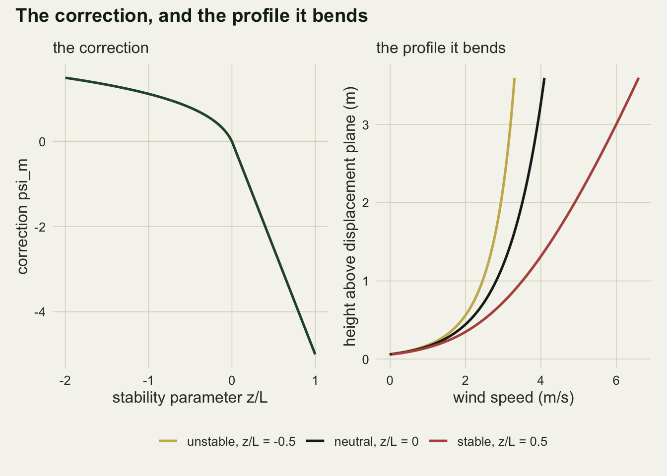
The footprint and its cumulative both have closed forms
Schuepp et al (1990) solved the diffusion equation for a scalar released at the surface and integrated across wind, and the answer is short enough to write on one line. With A the mean advection scale, the contribution of upwind distance x to the measured flux is
f(x) = (A / x^2) exp(-A / x)
and A = U z / (k u*), with U the layer-mean wind speed from the previous section. Everything a site wants to know follows from A alone. The cumulative has an elementary primitive: substituting u = A / x turns the integral into an exponential, so the fraction of the flux arriving from within x metres upwind is F(x) = exp(-A / x). The peak of f sits at x = A / 2, and inverting the cumulative gives the fetch containing a share p of the flux as -A / log(p). Those are algebraic identities rather than measurements, and worth checking against a numerical integration.
a_scale <- function(zz, zh = z_ref, z0 = z0_rough)
  zh * prof_term(zz, zh, z0) / k_von^2
a_scale_bar <- function(zz, zh = z_ref, z0 = z0_rough)
  zh * (log(zh / z0) - psi_bar(zz, zh) + z0 / zh - 1) / k_von^2
foot_dens <- function(xx, aa) (aa / xx^2) * exp(-aa / xx)
foot_cum  <- function(xx, aa) exp(-aa / xx)
fetch_at  <- function(pp, aa) -aa / log(pp)
a_neu <- a_scale(0); a_from_u <- u_bar_neu * z_ref / (k_von * us_check)
x_check  <- c(10, 25, 50, 100, 200, 400, 800)
cum_err  <- max(abs(vapply(x_check, function(xx)
  integrate(foot_dens, 1e-8, xx, aa = a_neu, rel.tol = 1e-10)$value,
  numeric(1)) - foot_cum(x_check, a_neu)))
peak_num <- optimize(foot_dens, c(1, 500), aa = a_neu, maximum = TRUE)$maximum
peak_err <- abs(peak_num - a_neu / 2)
share_mid <- 0.8; share_hi <- 0.9; f50 <- fetch_at(0.5, a_neu)
f80 <- fetch_at(share_mid, a_neu); f90 <- fetch_at(share_hi, a_neu)

print(round(c(advection_scale = a_neu, same_from_wind_speed = a_from_u,
  peak_numerical = peak_num, peak_analytic = a_neu / 2, fetch_50 = f50,
  fetch_80 = f80, fetch_90 = f90, fetch_90_over_50 = f90 / f50), 4))
advection_scale same_from_wind_speed peak_numerical
69.9466 69.9466 34.9733
peak_analytic fetch_50 fetch_80
34.9733 100.9116 313.4600
fetch_90 fetch_90_over_50
663.8785 6.5788 print(signif(c(max_cumulative_difference = cum_err, peak_diff = peak_err), 3))max_cumulative_difference peak_diff
5.55e-17 1.21e-05 Under neutral stratification this tower has an advection scale of 69.9 m. The chunk computes it twice, once from the layer-mean wind speed and the friction velocity and once from the height and roughness alone; both routes call the same profile term, so their agreement checks the substitution and nothing more. The two comparisons that follow are stronger, because they put the closed forms against a numerical integration: that integration of the density matches the closed-form cumulative to \(5.6 \times 10^{-17}\), and the numerically located peak sits \(1.2 \times 10^{-5}\) m from the analytic A / 2, both of which are numerical noise. Half the neutral flux arrives from within 101 m, 80 per cent from within 313 m, and 90 per cent from within 664 m. The last is 6.6 times the first, because the density decays only as the inverse square of distance, so a site that reports a single fetch number is choosing a quantile of a strongly skewed distribution.
Friction velocity cancels out of the source area
Now the step that decides what the rest of the post may claim. Substitute the profile into the definition of A:
A = U z / (k u*) = [ (u* / k) T(z/L) ] z / (k u*) = z T(z/L) / k^2
where T is the bracketed profile term, ln(z / z0) - psi_m + z0 / z - 1. The friction velocity appears once in the numerator and once in the denominator, and it is gone: under Monin-Obukhov similarity the source area depends on the height above the displacement plane, the roughness length and the stability, and on nothing else. Two half hours with the same stability and friction velocities differing by a factor of twenty have the same footprint, because the stronger wind that carries material further is produced by exactly the turbulence that mixes it down faster.
zeta_fix <- 0.2
us_sweep <- seq(0.05, 1.00, by = 0.005)
u_sweep  <- u_layer(us_sweep, zeta_fix)
a_sweep  <- u_sweep * z_ref / (k_von * us_sweep)
a_direct <- a_scale(zeta_fix)
u_span <- max(u_sweep) / min(u_sweep); a_dev <- max(abs(a_sweep / a_direct - 1))
x_span <- max(a_sweep / 2) - min(a_sweep / 2)
zeta_pair <- c(-0.3, 0.0, 0.3, 0.6); a_pair <- a_scale(zeta_pair)
print(round(c(friction_velocity_span = u_span, wind_low = min(u_sweep),
              wind_high = max(u_sweep), advection_scale = a_direct), 4))
friction_velocity_span wind_low wind_high
20.0000 0.5138 10.2762
advection_scale
92.4341 print(signif(c(max_relative_deviation = a_dev, peak_span_m = x_span), 3))max_relative_deviation peak_span_m
2.22e-16 2.13e-14 print(round(rbind(stability = zeta_pair, advection_scale = a_pair,
peak_distance = a_pair / 2), 2)) [,1] [,2] [,3] [,4]
stability -0.30 0.00 0.30 0.60
advection_scale 56.58 69.95 103.68 137.41
peak_distance 28.29 34.97 51.84 68.70Across friction velocities from 0.05 to 1.00 m/s, a span of 20, the layer-mean wind speed at fixed stability runs from 0.51 to 10.28 m/s, and the advection scale computed from that wind speed stays at 92.4 m throughout. The largest relative deviation over the sweep and the distance the peak contribution moves, both printed above, are floating-point rounding, not physics. Stability is what is left: moving the stability parameter from -0.3 to 0.6, which spans a mildly convective afternoon to a well stratified night at this height, takes the advection scale from 57 m to 137 m and the peak contribution distance from 28 m to 69 m. So the sentence “the retained night half hours have a smaller source area” cannot be derived from a friction velocity screen. It can only be true if calm half hours are more stable than windy ones, and that is a statement about the site’s weather, not about the footprint model. The next section puts that statement in explicitly, and the one after takes it out again.
What the screen keeps and what it discards
The simulated year is built the way the sibling posts build theirs: solar geometry from latitude and day of year, a clearness index that carries over from one day to the next, and a friction velocity with a synoptic component, a daytime convective boost and a penalty on clear nights. The stability parameter is then derived rather than drawn, because Monin-Obukhov similarity gives it: z / L = -k z g H / (rho cp T u*^3), with H the sensible heat flux. That derivation is where the assumption lives, and it should be named. The night-time downward heat flux is made to grow with friction velocity as u* to the power q, with q set to one, so that a windy night draws more heat down from aloft than a calm one. Since the stability parameter carries u* to the power minus three, the net dependence is u* to the power q - 3, which at q of one is the inverse square: calm nights are stable nights. That is a defensible description of a fen at night, it is the entire engine of the contrast below, and it is not a consequence of the footprint model.
g_acc <- 9.81; rho_air <- 1.2; cp_air <- 1005; t_kelvin <- 283.15
n_day <- 365; per_day <- 48; n_hh <- n_day * per_day
doy <- rep(seq_len(n_day), each = per_day)
hod <- rep(seq(0.25, 23.75, by = 0.5), n_day); lat_rad <- 47 * pi / 180
decl <- 23.44 * pi / 180 * sin(2 * pi * (doy - 81) / 365)
sin_elev <- sin(lat_rad) * sin(decl) +
  cos(lat_rad) * cos(decl) * cos((hod - 12) * 15 * pi / 180)
is_night <- sin_elev <= 0
h_night_ref <- 25; u_ref <- 0.25; q_base <- 1; h_day_max <- 230
zeta_target <- 0.10; zeta_cap <- 1.0; zeta_cap_un <- 2.0

sim_year <- function(seed, q_pow = q_base) {
  set.seed(seed)
  kt <- numeric(n_day); kt[1] <- 0.6
  for (dd in 2:n_day) kt[dd] <- 0.58 + 0.55 * (kt[dd - 1] - 0.58) +
    rnorm(1, 0, 0.17)
  clr <- rep(pmin(0.95, pmax(0.16, kt)), each = per_day)
  syn <- rep(as.numeric(stats::filter(rnorm(n_day, 0, 0.30), 0.70,
                                      method = "recursive")), each = per_day)
  eps <- as.numeric(stats::filter(rnorm(n_hh, 0, 0.12), 0.85,
                                  method = "recursive"))
  us <- pmin(pmax(exp(log(0.30) + 0.50 * pmax(0, sin_elev)^0.6 + syn -
                        0.35 * clr * is_night + eps), 0.03), 1.5)
  hf <- ifelse(is_night,
               -h_night_ref * (0.35 + 0.65 * clr) * (us / u_ref)^q_pow,
               h_day_max * pmax(0, sin_elev) * (0.25 + 0.75 * clr))
  to_zeta <- function(hh)
    -k_von * z_ref * g_acc * hh / (rho_air * cp_air * t_kelvin * us^3)
  hf[is_night] <- hf[is_night] * (zeta_target / median(to_zeta(hf)[is_night]))
  zr <- to_zeta(hf)
  data.frame(ustar = us, heat = hf, zeta_raw = zr,
             zeta = pmin(pmax(zr, -zeta_cap_un), zeta_cap))
}

u_thr <- 0.20; r_field <- 150
class_of <- function(us, thr = u_thr) ifelse(!is_night, "day",
  ifelse(us >= thr, "night retained", "night discarded"))
yr_one <- sim_year(20260810); p_tail <- 0.05
heat_p05 <- unname(quantile(yr_one$heat[is_night], p_tail))
pin_day <- mean(yr_one$zeta_raw[!is_night] < -zeta_cap_un)
pin_night <- mean(yr_one$zeta_raw[is_night] > zeta_cap)
print(round(c(half_hours = n_hh, night_share = mean(is_night),
  night_ustar_median = median(yr_one$ustar[is_night]),
  night_heat_median = median(yr_one$heat[is_night]), night_heat_5th = heat_p05,
  night_zeta_median = median(yr_one$zeta[is_night]),
  day_zeta_median = median(yr_one$zeta[!is_night]),
  day_pinned_unstable = pin_day, night_pinned_stable = pin_night), 4))
half_hours night_share night_ustar_median night_heat_median
17520.0000 0.5000 0.2428 -34.1510
night_heat_5th night_zeta_median day_zeta_median day_pinned_unstable
-74.0272 0.1000 -0.0372 0.0039
night_pinned_stable
0.0066 The year has 17520 half hours, 50 per cent of them at night. The median night-time friction velocity is 0.243 m/s, the median night-time sensible heat flux -34.2 W/m2 and the median night-time stability parameter 0.100, against -0.037 by day. Those are ordinary values for a low mast over short vegetation, where the stability parameter is small largely because the measurement height is small. The tail of the heat flux is not ordinary: 5 per cent of night half hours carry a downward flux stronger than 74 W/m2, which is high for a wet fen, and it comes from forcing the median night-time stability to a target rather than from anything measured. Now the screen and the three classes it creates, with every quantity below a mean over the half hours in a class, averaged again over independently simulated years so that it carries a Monte Carlo standard error.
summarise_year <- function(yr, thr = u_thr, rr = r_field,
                           zh = z_ref, z0 = z0_rough, afun = a_scale) {
  aa <- afun(yr$zeta, zh, z0)
  cl <- class_of(yr$ustar, thr)
  c(A_day = mean(aa[cl == "day"]), A_keep = mean(aa[cl == "night retained"]),
    A_drop = mean(aa[cl == "night discarded"]),
    F_day = mean(foot_cum(rr, aa[cl == "day"])),
    F_keep = mean(foot_cum(rr, aa[cl == "night retained"])),
    F_drop = mean(foot_cum(rr, aa[cl == "night discarded"])),
    drop_share = mean(yr$ustar[is_night] < thr))
}

n_rep <- 60; seed_set <- 20260810 + seq_len(n_rep)
rep_mat <- vapply(seed_set, function(s) summarise_year(sim_year(s)), numeric(7))
est <- rowMeans(rep_mat); mcse <- apply(rep_mat, 1, sd) / sqrt(n_rep)
peak_keep <- est[["A_keep"]] / 2; peak_drop <- est[["A_drop"]] / 2
gap_yr <- rep_mat["F_keep", ] - rep_mat["F_drop", ]
f_gap <- mean(gap_yr); gap_sd <- sd(gap_yr); f_gap_se <- gap_sd / sqrt(n_rep)
a_bar_fix <- a_scale_bar(zeta_fix)
bar_mat <- vapply(seed_set, function(s) summarise_year(sim_year(s),
  afun = a_scale_bar)[c("F_keep", "F_drop")], numeric(2))
gap_bar <- mean(bar_mat["F_keep", ] - bar_mat["F_drop", ])

print(round(rbind(estimate = est, monte_carlo_se = mcse), 4))
A_day A_keep A_drop F_day F_keep F_drop drop_share
estimate 65.1231 77.8192 107.448 0.6483 0.5955 0.4942 0.3472
monte_carlo_se 0.0725 0.0890 0.491 0.0003 0.0003 0.0015 0.0061print(round(c(replicate_years = n_rep, peak_retained = peak_keep,
peak_discarded = peak_drop, peak_ratio = peak_drop / peak_keep,
fraction_gap = f_gap, fraction_gap_se = f_gap_se, gap_year_low = min(gap_yr),
gap_year_high = max(gap_yr), gap_year_sd = gap_sd, gap_psi_averaged = gap_bar,
advection_psi_averaged = a_bar_fix,
day_over_discarded = est[["A_drop"]] / est[["A_day"]]), 4)) replicate_years peak_retained peak_discarded
60.0000 38.9096 53.7240
peak_ratio fraction_gap fraction_gap_se
1.3807 0.1013 0.0013
gap_year_low gap_year_high gap_year_sd
0.0834 0.1273 0.0097
gap_psi_averaged advection_psi_averaged day_over_discarded
0.0559 81.1903 1.6499 Over 60 simulated years the screen removes 34.7 per cent of night-time half hours, with a Monte Carlo standard error of 0.6 percentage points. The half hours it keeps have a mean advection scale of 77.8 m and the ones it discards 107.4 m, against 65.1 m by day. In distance of peak contribution that is 39 m for the retained night half hours and 54 m for the discarded ones, a ratio of 1.38.
Put a field boundary 150 m upwind, which for this fen is where the sedge gives way to drained grassland. 64.8 per cent of the daytime flux comes from inside it, 59.6 per cent of the retained night-time flux and 49.4 per cent of the discarded night-time flux, the largest of the three Monte Carlo standard errors being 0.15 percentage points. The gap between the two night classes is 10.1 percentage points with a Monte Carlo standard error of 0.13, so it is far larger than the simulation noise on it. Changing the whole seed set moves the class means by about those standard errors, but a single year is a far coarser instrument: across the 60 years the gap runs from 8.3 to 12.7 percentage points with a standard deviation of 0.97, so one simulated year settles the sign of the gap but not its size.
cls_lab <- c("day", "night retained", "night discarded")
pan_fp <- c("contribution per metre", "cumulative share of the flux")
a_cls <- c(est[["A_day"]], est[["A_keep"]], est[["A_drop"]])
x_dist <- seq(2, 600, length.out = 500)
fp_dat <- do.call(rbind, Map(function(av, lb) data.frame(
  x = x_dist, y = c(foot_dens(x_dist, av), foot_cum(x_dist, av)),
  cls = factor(lb, levels = cls_lab),
  panel = factor(rep(pan_fp, each = length(x_dist)), levels = pan_fp)),
  a_cls, cls_lab))
cross_dat <- data.frame(x = r_field, y = foot_cum(r_field, a_cls),
  cls = factor(cls_lab, levels = cls_lab),
  panel = factor(pan_fp[2], levels = pan_fp))
ggplot(fp_dat, aes(x, y, colour = cls)) +
  geom_vline(xintercept = r_field, linetype = "22", colour = te_body,
             linewidth = 0.5) +
  geom_line(linewidth = 0.9) + geom_point(data = cross_dat, size = 2.8) +
  facet_wrap(~panel, scales = "free_y") +
  scale_colour_manual(values = c(te_forest, te_gold, te_rust), name = NULL) +
  labs(x = "upwind distance (m)", y = NULL,
       title = "Where the flux comes from, and how much is inside the field",
       subtitle = "dashed line: the field boundary at 150 m") +
  theme_datasheet() +
  theme(legend.position = "bottom",
        strip.text = element_text(colour = te_ink, face = "bold"))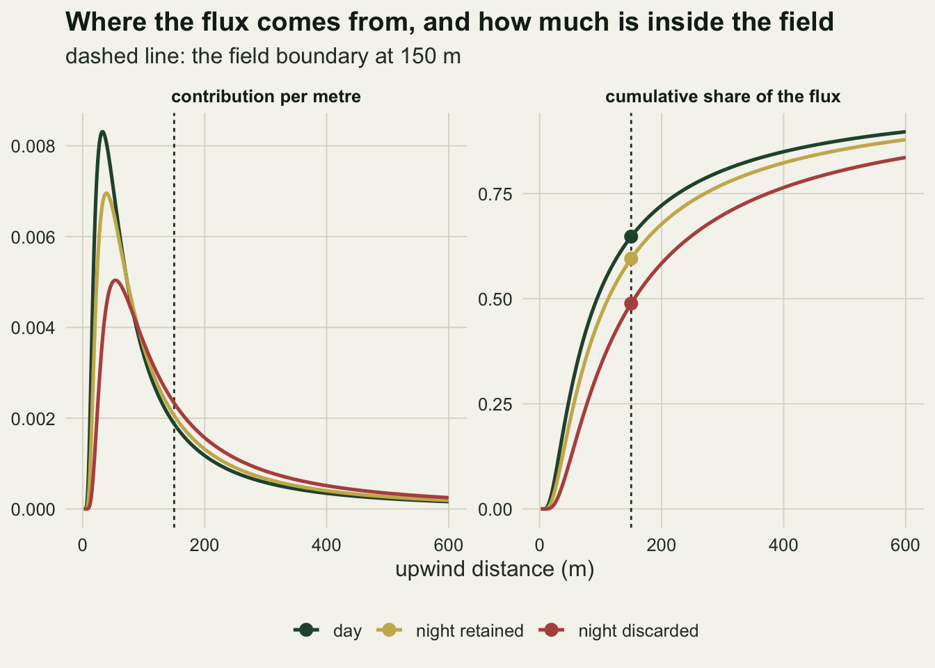
The direction of the contrast is an assumption, not a physical law
The exponent q tying the night-time heat flux to the friction velocity was set to one and never questioned. It is the main thing making calm nights stable, and stability is the only thing moving the footprint, so the result stands or falls with it. The test is to push it to the other end: holding the median night-time stability fixed by recalibrating the heat flux each time, vary q from zero, where the heat flux ignores the wind and the stability parameter falls as the inverse cube of friction velocity, up to five, where windy nights become the stratified ones.
q_grid <- c(0, 1, 2, 3, 4, 5)
n_rep_q <- 25
q_res <- t(vapply(q_grid, function(qq) {
  gapv <- numeric(n_rep_q); corv <- numeric(n_rep_q); xgv <- numeric(n_rep_q)
  for (j in seq_len(n_rep_q)) {
    yy <- sim_year(seed_set[j], q_pow = qq)
    ss <- summarise_year(yy)
    gapv[j] <- ss[["F_keep"]] - ss[["F_drop"]]
    xgv[j]  <- (ss[["A_drop"]] - ss[["A_keep"]]) / 2
    corv[j] <- cor(log(yy$ustar[is_night]), log(yy$zeta[is_night]))
  }
  c(q = qq, corr = mean(corv), gap = mean(gapv),
    gap_se = sd(gapv) / sqrt(n_rep_q), peak_gap = mean(xgv))
}, numeric(5)))
q_tab <- as.data.frame(q_res)
print(round(q_tab, 4))
q corr gap gap_se peak_gap
1 0 -0.9845 0.1582 0.0025 24.7304
2 1 -0.9833 0.0997 0.0018 14.5485
3 2 -0.9442 0.0423 0.0007 5.6450
4 3 -0.1297 0.0016 0.0002 0.2121
5 4 0.9333 -0.0324 0.0005 -4.2485
6 5 0.9820 -0.0710 0.0012 -9.9422q_max <- q_tab$gap[q_tab$q == 0]; q_flip <- q_tab$gap[q_tab$q == 5]
q_def <- q_tab$gap[q_tab$q == q_base]
q_zero <- q_tab$gap[q_tab$q == 3]; q_zero_se <- q_tab$gap_se[q_tab$q == 3]
peak_flip <- q_tab$peak_gap[q_tab$q == 5]The direction flips, and each point below is the mean over 25 simulated years. At q of zero the correlation between log friction velocity and log stability across night half hours is -0.98, and the retained half hours draw 15.8 percentage points more of their flux from inside the field boundary than the discarded ones. At q of three the exponent on friction velocity is zero, the correlation collapses to -0.13 and the gap falls to 0.16 percentage points with a standard error of 0.02. At q of five the correlation is 0.98, the gap is -7.1 percentage points, and the peak contribution of the retained half hours lies 10 m further upwind than that of the discarded ones. The screen now selects the longer fetch rather than the shorter one.
The residual at q of three is the interesting part. The gap does not cross zero at the exponent where the algebra cancels but a little above it, because clear skies both suppress the friction velocity and deepen the radiative heat loss, so a second and weaker path from turbulence to stability survives when the direct one is switched off. That leftover is 0.16 percentage points against 10.0 at the default coupling of q equal to 1, the dashed line in the figure below, and 15.8 at the strongest coupling tried: real, and small. None of this says the effect is imaginary. It says the sign and size of the spatial bias are properties of the local coupling between turbulence and stratification, measurable at any tower that logs a sonic temperature covariance, and not properties of the screen. A site that reports the bias without reporting the coupling has reported half a result.
pan_cp <- c("correlation of log u-star and log z/L",
            "retained minus discarded (percentage points)")
cp_dat <- data.frame(
  q = rep(q_tab$q, 2), y = c(q_tab$corr, 100 * q_tab$gap),
  lo = c(q_tab$corr, 100 * (q_tab$gap - 2 * q_tab$gap_se)),
  hi = c(q_tab$corr, 100 * (q_tab$gap + 2 * q_tab$gap_se)),
  panel = factor(rep(pan_cp, each = nrow(q_tab)), levels = pan_cp))
ggplot(cp_dat, aes(q, y, colour = panel)) +
  geom_hline(yintercept = 0, colour = te_line, linewidth = 0.6) +
  geom_vline(xintercept = q_base, linetype = "22", colour = te_body,
             linewidth = 0.5) +
  geom_errorbar(aes(ymin = lo, ymax = hi), width = 0.12, linewidth = 0.6) +
  geom_line(linewidth = 0.9) + geom_point(size = 2.6) +
  facet_wrap(~panel, ncol = 1, scales = "free_y") +
  scale_y_continuous(breaks = function(lims) pretty(lims, 6)) +
  scale_colour_manual(values = c(te_forest, te_rust), guide = "none") +
  labs(x = "exponent q in night-time heat flux proportional to u-star^q",
       y = NULL, title = "Turn the coupling around and the result turns with it",
       subtitle = "dashed line: the exponent used in the section above") +
  theme_datasheet() +
  theme(strip.text = element_text(colour = te_ink, face = "bold"))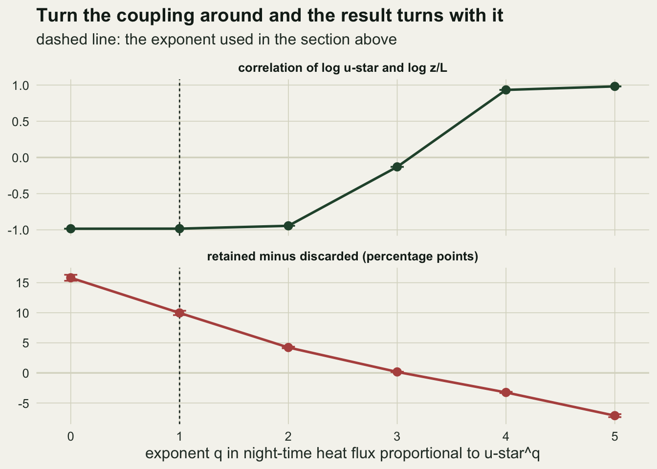
Four fixed numbers were choices
Every design parameter above was set once and then treated as a fact. There are four: the measurement height of four metres, the canopy height that fixes both the roughness length and the displacement height, the friction velocity threshold of 0.20 m/s, and the field boundary at 150 m. Freeing them one at a time says which of them the answer is sensitive to. All four sweeps run on the single simulated year above rather than on the sixty-year set, so each gap below carries year-to-year noise of the same order as the spread quoted earlier. Raising the mast is not a change of height alone either. The stability parameter is z / L, and L is a property of the surface and the fluxes rather than of the sensor, so a sonic at twice the height sits at twice the stability parameter on the same night. Holding z / L fixed while the mast grows measures nothing physical, and the sweep below rescales it with height; the canopy sweep needs the same treatment, because moving the displacement plane moves the height that enters z / L too.
mast_set <- c(2, 4, 6, 8, 16); thr_set <- c(0.10, 0.15, 0.20, 0.25, 0.30)
fld_set <- c(50, 100, 150, 300, 600); can_set <- c(0.05, 0.20, 0.60, 1.20)
sweep_rows <- function(nm, vals, ovr) do.call(rbind, lapply(vals, function(v) {
  argl <- list(yr = yr_one, thr = u_thr, rr = r_field, zh = z_ref, z0 = z0_rough)
  argl[names(ovr(v))] <- ovr(v)
  ss <- do.call(summarise_year, argl)
  data.frame(parameter = nm, value = v, A_keep = ss[["A_keep"]],
             A_drop = ss[["A_drop"]], discarded = ss[["drop_share"]],
             gap = ss[["F_keep"]] - ss[["F_drop"]])
}))
design <- rbind(
  sweep_rows("mast", mast_set, function(v) list(zh = v - d_disp)),
  sweep_rows("canopy", can_set, function(v)
    list(zh = z_meas - 0.67 * v, z0 = 0.1 * v)),
  sweep_rows("threshold", thr_set, function(v) list(thr = v)),
  sweep_rows("boundary", fld_set, function(v) list(rr = v)))
gap_rng <- tapply(design$gap, design$parameter, function(v) diff(range(v)))

zeta_night <- yr_one$zeta[is_night]
cap_frac <- vapply(mast_set, function(v)
  mean(zeta_night * (v - d_disp) / z_ref > zeta_cap), numeric(1))
cap_max <- max(zeta_night * (mast_set[length(mast_set)] - d_disp) / z_ref)
zeta_demo <- 1.5
a_uncapped <- a_scale(zeta_demo); a_capped <- a_scale(zeta_cap)
print(round(design[, -1], 4)); print(round(gap_rng, 4))
value A_keep A_drop discarded gap
1 2.00 24.6900 30.1793 0.3438 0.0302
2 4.00 77.6618 105.4903 0.3438 0.0966
3 6.00 142.7608 210.1257 0.3438 0.1285
4 8.00 217.1938 341.2921 0.3438 0.1187
5 16.00 589.9705 1112.9748 0.3438 0.0205
6 0.05 150.1243 183.9450 0.3438 0.0705
7 0.20 112.0672 144.1957 0.3438 0.0869
8 0.60 77.6618 105.4903 0.3438 0.0966
9 1.20 52.4237 74.3811 0.3438 0.0926
10 0.10 85.0910 158.0072 0.0293 0.2179
11 0.15 81.0515 121.8089 0.1516 0.1346
12 0.20 77.6618 105.4903 0.3438 0.0966
13 0.25 75.4051 98.0424 0.5224 0.0805
14 0.30 74.0417 94.0264 0.6599 0.0720
15 50.00 77.6618 105.4903 0.3438 0.0822
16 100.00 77.6618 105.4903 0.3438 0.1052
17 150.00 77.6618 105.4903 0.3438 0.0966
18 300.00 77.6618 105.4903 0.3438 0.0668
19 600.00 77.6618 105.4903 0.3438 0.0393 boundary canopy mast threshold
0.0659 0.0261 0.1080 0.1459 print(round(c(cap_exceeded = cap_frac, max_effective_zeta = cap_max,
advection_uncapped = a_uncapped, advection_capped = a_capped), 3)) cap_exceeded1 cap_exceeded2 cap_exceeded3 cap_exceeded4
0.000 0.000 0.026 0.055
cap_exceeded5 max_effective_zeta advection_uncapped advection_capped
0.195 4.335 238.603 182.384 pick <- function(nm, col) design[[col]][design$parameter == nm]
mast_a <- pick("mast", "A_keep"); mast_gap <- pick("mast", "gap")
thr_gap <- pick("threshold", "gap"); thr_drop <- pick("threshold", "discarded")
fld_gap <- pick("boundary", "gap"); can_gap <- pick("canopy", "gap")
can_a <- pick("canopy", "A_keep"); can_z0 <- 0.1 * can_setThe mast height is by far the strongest lever on the footprint itself. Raising the sensor from 2 m to 16 m takes the retained-class advection scale from 25 m to 590 m, a factor of 23.9, because the scale is height times a bracket that itself grows with height, through the logarithm and through the stability term together. Its effect on the retained-minus-discarded gap is not monotonic: the gap is 3.0 percentage points on a 2 m mast, widest at 12.8 on the 6 m mast, which is the turning point among the heights tried, and 2.0 on a 16 m one, where the whole footprint has moved out past the boundary in every class. The 4 m mast used through the post gives 9.7, on the near side of the turning point rather than at it. Rescaling the stability parameter with height also carries the sweep past the cap named in Honest limits, which binds at the reference height only: the effective value exceeds it on 2.6 per cent of night half hours at 6 m, 5.5 per cent at 8 m and 19.5 per cent at 16 m, reaching 4.34, so the tallest row is largely extrapolation of a linear stable term well past the range it was fitted over.
The friction velocity threshold is the parameter the gap is most sensitive to over the windows swept here: its range of 14.6 percentage points is the widest of the four, against 10.8 for the mast, 6.6 for the boundary and 2.6 for the canopy. That ranking is as much a statement about the swept windows as about the parameters. Moving the threshold from 0.10 to 0.30 m/s takes the gap from 21.8 percentage points down to 7.2. A low threshold discards 2.9 per cent of night half hours, only the calmest and most stratified tail, where the footprint is most stretched, so the two classes are at their most different; a high one discards 66.0 per cent, a broad slice of ordinary nights, and the classes look alike. The size of the spatial selection is set by the threshold, which is itself estimated from the data and carries the downward bias the u-star post measured.
The canopy is the one design number a site can measure rather than choose, and it moves two things at once: the roughness length, a tenth of the canopy here, and the displacement height, two thirds of it. Across canopies from 0.05 m to 1.20 m, that is roughness lengths of 0.005 to 0.12 m, the retained-class advection scale falls from 150 m to 52 m while the gap only runs from 7.0 to 9.7 percentage points. The field boundary is a reporting choice rather than a site property, and the gap is not monotonic in it either: 8.2 percentage points at 50 m, a maximum of 10.5 at 100 m, and 3.9 at 600 m. A boundary drawn very close in captures little of any class and one far out in the tail captures nearly all of every class, so the classes separate only in between: quoting the gap at one distance is quoting one point on a curve.
What to report
Report the source area, not just a fetch, and report it by stability class. The advection scale determines the whole crosswind-integrated footprint under this model: the peak distance is half of it and the fetch containing any share is minus it divided by the log of that share, so quoting it alongside the measurement height, the roughness length and the stability distribution lets a reader reconstruct whatever quantile they want. A single annual figure averages a compact convective daytime footprint with a stretched nocturnal one, and the daytime mean here differs from the discarded night-time mean by a factor of 1.65 in advection scale. If the record has been through a friction velocity screen, give the fetch of the retained half hours separately from the fetch of everything, because those are the half hours that survive into the budget.
State the coupling between friction velocity and stability at the site, as a correlation or a fitted exponent, whenever a spatial claim is made about the screen. It decides the sign, it is measurable from the same sonic anemometer that produces the flux, and without it the claim that a screen selects a smaller source area is unsupported. Papale et al (2006) fixed the processing convention for the screen; nothing in that convention constrains where the surviving half hours came from.
Give the design parameters that went into the footprint: the measurement height above the displacement plane rather than above the ground, the roughness length and how it was obtained, the stability range over which the profile functions were applied, and the distance at which any percentage was evaluated. Many disagreements between published fetch figures for similar sites are differences in these rather than differences in the sites.
Honest limits
The footprint model is the simplest one with a closed form. Schuepp et al (1990) assume a constant eddy diffusivity through the layer and no crosswind spread, which is what makes the analytical work possible and the answer approximate. Horst and Weil (1992) showed that a height-dependent diffusivity moves the peak and changes the shape of the tail, Kormann and Meixner (2001) give a power-law diffusivity solution valid across stabilities, and Kljun et al (2015) provide a two-dimensional parameterisation fitted to Lagrangian simulations, which is what a real site should use. Every distance in this post would shift under those; the statement about stability would not. The crosswind integration is a further loss rather than a technicality: what is computed is the share arriving from within a given distance upwind, not the share arriving from within a circle or a field of a given shape. A boundary at a fixed distance is a boundary in one wind direction only, and at a site where the wind veers between day and night the contrast in what is actually sampled could be larger or smaller than the contrast in fetch. Goeckede et al (2008) coupled footprint calculations to wind direction and terrain for exactly this reason when screening flux sites for data quality.
The stability correction is used at the edge of what it was built for, and it carries two conventions worth naming. The Dyer relation was established over conditions from near neutral to moderately stable and is known to fail in strong stability, which is where the half hours the screen removes live, so the stability parameter was capped at 1.0 on the stable side and at minus 2.0 on the unstable side; those caps bind on 0.66 per cent of night half hours and 0.39 per cent of day half hours in the year above, and they are limits of the parameterisation rather than of the profile, since wind speed rises with height at every positive L. The second convention sits inside the bracket, where the log terms are depth-averaged over the layer but psi_m is taken at the measurement height. The two errors run in opposite directions and each keeps its own sign. Capping shortens the most stratified half hours: at a stability parameter of 1.5 the uncapped advection scale is 239 m and the cap holds it to 182 m, so the cap understates how far upwind those half hours reach. The published bracket stretches them instead: averaging the correction over the same layer halves it exactly on the stable side, takes the advection scale at a stability parameter of 0.2 from 92.4 m down to 81.2 m, and puts the headline gap at 5.6 percentage points instead of 10.1. The headline number is therefore conditional on a convention as well as on a simulation.
The simulated joint distribution of friction velocity and stability is a construction, and two sections above exist because of it. Nothing was fitted to a real fen: the exponent tying the night-time heat flux to friction velocity was chosen, the clearness process was chosen, and the reported gap of 10.1 percentage points is a statement about that construction. What survives outside it is the algebra: the cancellation of friction velocity, the closed-form cumulative, and the finding that the direction of the contrast is decided by a correlation any tower can measure and few report. Finally, a screened flux record has a spatial bias but this post does not price it in carbon. Whether the ground the retained half hours over-sample respires more or less than the ground they under-sample depends on the site, and on a homogeneous fen it does not matter at all. It matters in the common case: a tower at the edge of the ecosystem it was meant to measure, where the stretched nocturnal footprint reaches across the boundary and the compact daytime one does not.
References
Schuepp PH, Leclerc MY, MacPherson JI, Desjardins RL 1990 Boundary-Layer Meteorology 50(1-4):355-373 (10.1007/BF00120530)
Horst TW, Weil JC 1992 Boundary-Layer Meteorology 59(3):279-296 (10.1007/BF00119817)
Kormann R, Meixner FX 2001 Boundary-Layer Meteorology 99(2):207-224 (10.1023/A:1018991015119)
Kljun N, Calanca P, Rotach MW, Schmid HP 2015 Geoscientific Model Development 8(11):3695-3713 (10.5194/gmd-8-3695-2015)
Paulson CA 1970 Journal of Applied Meteorology 9(6):857-861 (10.1175/1520-0450(1970)009<0857:TMROWS>2.0.CO;2)
Dyer AJ 1974 Boundary-Layer Meteorology 7(3):363-372 (10.1007/BF00240838)
Papale D, Reichstein M, Aubinet M, Canfora E, Bernhofer C, Kutsch W, Longdoz B, Rambal S, Valentini R, Vesala T, Yakir D 2006 Biogeosciences 3(4):571-583 (10.5194/bg-3-571-2006)
Goeckede M, Foken T, Aubinet M, Aurela M, Banza J, Bernhofer C, Bonnefond JM, Brunet Y, Carrara A, Clement R, Dellwik E, Elbers J, et al 2008 Biogeosciences 5(2):433-450 (10.5194/bg-5-433-2008)