library(ggplot2)

te_pal <- list(forest = "#275139", green = "#2f8f63", sage = "#93a87f",
               clay = "#b5534e", gold = "#cda23f", line = "#dad9ca",
               ink = "#16241d", paper = "#f5f4ee")

theme_te <- function() {
  theme_minimal(base_size = 12) +
    theme(panel.grid.minor = element_blank(),
          panel.grid.major = element_line(colour = "#e7e6dc"),
          plot.background = element_rect(fill = "#f5f4ee", colour = NA),
          panel.background = element_rect(fill = "#f5f4ee", colour = NA),
          plot.title = element_text(face = "bold", colour = te_pal$ink),
          axis.title = element_text(colour = "#2c3a31"),
          axis.text = element_text(colour = "#2c3a31"))
}Partitioning net flux into GPP and respiration
R
eddy covariance
carbon flux
GPP
ecology tutorial
Splitting eddy covariance net flux into GPP and ecosystem respiration in R: why both gross fluxes go wrong together while the annual net total stays right.
A flux tower stands over a mixed deciduous stand at a little under fifty degrees north. The sonic anemometer and the gas analyser sit above the canopy, the raw twenty-hertz data get averaged into half-hourly covariances, and one calendar year of that is seventeen and a half thousand rows in a spreadsheet. The column that matters is net ecosystem exchange: the sum of everything the ecosystem released and everything it took up in each half hour. Negative means the ecosystem was a sink in that half hour, positive means it was a source, and that sign convention is a choice the community made rather than a fact, so it gets stated once and kept.
The year has already been through two steps before this post starts. Calm nights have been screened out with a friction velocity threshold, because on a still night the turbulence that the method depends on is not there and the tower measures a flux that went sideways instead of up. The holes that screening leaves, along with the rain outages and the calibration gaps, have been filled. Those two steps are covered separately in night-time flux and the u-star threshold and gap filling a flux time series; everything below assumes they are done and takes the filled series as given.
What the tower did not measure, and cannot measure, is either of the two fluxes that almost every paper using the data goes on to report. Gross primary production is the carbon fixed by photosynthesis. Ecosystem respiration is the carbon released by leaves, roots, wood and soil microbes. The tower sees only their difference. Getting the two gross numbers out of the one net number is called partitioning, and it is not a measurement: it is a model fitted to one part of the data and then evaluated somewhere else.
That last clause is what this post is about, and it is what separates it from the two posts whose machinery it borrows. Nonlinear regression in R with nls and fitting growth curves with nls fit a curve through data and read parameters off it, and the fitted curve is checked against the points it was fitted to. Here the curve is fitted to night-time data and then evaluated in the daytime, where there are no respiration data at all and never will be, because in the light the two fluxes are happening at once and only their sum leaves the canopy. Extrapolation is the whole exercise, and extrapolation is the whole risk. The closest relative on this blog is the recalcitrant pool and the asymptote, where a litter decay model reports a limit value that no litterbag ever weighed: same logic, different substrate, and in both cases the model decides the number rather than the data.
Everything below runs on a simulated year with a truth column for both gross fluxes, so that every error is a distance from a value that was set rather than an argument about what should have happened. The simulation carries one piece of physiology that makes the extrapolation fail in a specific, measurable direction: leaf respiration is partly switched off in the light. Six things get measured: what the night-time fit recovers, what the extrapolation does to the annual totals, how the two errors relate to each other, what a daytime-based alternative buys, what an assumed temperature sensitivity is worth, and what happens when the fit is allowed to move through the season.
A year with a truth column
The drivers come first: solar geometry from the latitude and the day of year, a cloud factor that varies day to day, and an air temperature with a seasonal swing, a diurnal swing whose amplitude is itself larger in summer, and a daily weather anomaly on top.
lat_deg <- 47
n_day <- 365
doy <- rep(seq_len(n_day), each = 48)
hh <- rep(seq(0, 23.5, by = 0.5), times = n_day)
n_hh <- length(doy)

decl <- 23.45 * sin(2 * pi * (284 + doy) / 365) * pi / 180
lat_r <- lat_deg * pi / 180
hang <- 15 * (hh - 12) * pi / 180
sin_elev <- sin(lat_r) * sin(decl) + cos(lat_r) * cos(decl) * cos(hang)

set.seed(20260802)
cloud_day <- pmin(1, pmax(0.22, rbeta(n_day, 5, 1.8)))
cloud <- rep(cloud_day, each = 48) * runif(n_hh, 0.85, 1.05)
ppfd <- pmax(0, 2050 * pmax(0, sin_elev) * pmin(1, cloud))

day_anom <- rep(rnorm(n_day, 0, 2.6), each = 48)
tair <- 9.2 + 10.4 * sin(2 * pi * (doy - 112) / 365) + day_anom +
  (4.2 + 1.8 * sin(2 * pi * (doy - 112) / 365)) *
    sin(2 * pi * (hh - 9.5) / 24) + rnorm(n_hh, 0, 0.7)
tk <- tair + 273.15
lai <- 0.06 + 0.94 * exp(-((doy - 190) / 66)^2)

print(c(half_hours = n_hh, days = n_day, latitude = lat_deg))
half_hours days latitude
17520 365 47 print(round(c(min_temp = min(tair), mean_temp = mean(tair),
max_temp = max(tair), max_ppfd = max(ppfd),
peak_leaf_area = max(lai)), 2)) min_temp mean_temp max_temp max_ppfd peak_leaf_area
-10.15 9.05 31.38 1836.79 1.00 The year holds 17520 half hours at a latitude of 47 degrees north, air temperature runs from -10.15 to 31.38 degrees C with a mean of 9.05, and photosynthetic photon flux density peaks at 1836.8 umol/m2/s. Leaf area follows a bell through the summer with a small evergreen floor in winter.
Ecosystem respiration follows Lloyd and Taylor (1994), which writes the temperature response as
\[R(T) = R_{\text{ref}} \exp\left[E_0\left(\frac{1}{T_{\text{ref}} - T_0} - \frac{1}{T - T_0}\right)\right]\]
with temperatures in kelvin, a reference temperature of ten degrees C, a lower limit \(T_0\) that the original paper fixed at a value well below freezing and that everyone since has held there, a basal rate \(R_{\text{ref}}\) at the reference temperature, and an activation-energy parameter \(E_0\) that controls how steeply respiration climbs. Two departures from the textbook form go into the truth. The basal rate is not constant through the year: it rises with leaf area and with the fine-root and litter turnover that comes with it, so the temperature response is not stationary. And leaf respiration is partly inhibited in the light, an effect known from leaf-level work as the Kok effect and shown at whole-ecosystem scale by Wehr et al (2016), so daytime respiration is lower than a night-time relationship evaluated at the same temperature would predict.
tref_k <- 283.15
t0_k <- 227.13
lt_shape <- function(tkv, e0) {
  exp(e0 * (1 / (tref_k - t0_k) - 1 / (tkv - t0_k)))
}

rref_true <- 2.80
e0_true <- 208
seas_r <- 0.72 + 0.58 * lai
reco_pot <- rref_true * seas_r * lt_shape(tk, e0_true)

f_leaf <- 0.50 * lai
kok <- 0.60
light_sw <- ppfd / (ppfd + 25)
inhib <- kok * f_leaf * light_sw
reco_true <- reco_pot * (1 - inhib)

alpha_true <- 0.048
amax_true <- 26
gpp_true <- alpha_true * ppfd * (amax_true * lai) /
  (alpha_true * ppfd + amax_true * lai + 1e-9)
gpp_true[ppfd <= 0] <- 0

nee_true <- reco_true - gpp_true

set.seed(20260803)
sd_hh <- 0.55 + 0.115 * abs(nee_true)
nee_obs <- nee_true + rnorm(n_hh, 0, sd_hh)

gc_hh <- 12.011 * 1e-6 * 1800
ann <- function(x) sum(x) * gc_hh
night <- ppfd < 5
day_i <- which(!night)

gpp_ann <- ann(gpp_true)
reco_ann <- ann(reco_true)
nee_ann <- ann(nee_true)
kok_ann <- ann(reco_pot - reco_true)
inhib_pct <- 100 * sum(inhib[!night] * reco_pot[!night]) /
  sum(reco_pot[!night])

print(round(c(rref = rref_true, e0 = e0_true, alpha = alpha_true,
              amax = amax_true, kok_fraction = kok), 3))
rref e0 alpha amax kok_fraction
2.800 208.000 0.048 26.000 0.600 print(round(c(gpp_gc = gpp_ann, reco_gc = reco_ann, nee_gc = nee_ann,
kok_cost_gc = kok_ann, daytime_inhibition_pct = inhib_pct,
night_half_hours = sum(night), peak_reco = max(reco_true)), 2)) gpp_gc reco_gc nee_gc
1297.22 969.48 -327.73
kok_cost_gc daytime_inhibition_pct night_half_hours
116.34 17.56 8786.00
peak_reco
8.72 Gross primary production is a rectangular hyperbola in light with a saturating rate that scales with leaf area, so photosynthesis is zero at night by construction. Measurement noise is heteroscedastic, growing with the size of the flux, which is what flux errors actually do. The conversion from umol/m2/s to grams of carbon per half hour is one multiplication by 0.0216198.
The truth for the year: gross primary production 1297.2 gC/m2/yr, ecosystem respiration 969.5 gC/m2/yr, and net ecosystem exchange -327.7 gC/m2/yr, a sink of moderate strength for a temperate forest. The light inhibition of leaf respiration removes 17.56 per cent of daytime respiration on average and 116.3 gC/m2/yr over the year. That figure is the target: an extrapolation from the night has no way of knowing about it, so if nothing else went wrong the night-time method should overshoot annual respiration by about that much.
Of the 17520 half hours, 8786 fall below the light threshold and count as night. Those, and only those, are the data the standard method fits.
The night-time fit
The night-time method, set out in its modern form by Reichstein et al (2005), rests on one sentence: at night there is no photosynthesis, so net ecosystem exchange is respiration. That sentence is an assumption, not a measurement. Nothing in the data confirms it; it is believed because photosystems need photons. Everything downstream inherits it.
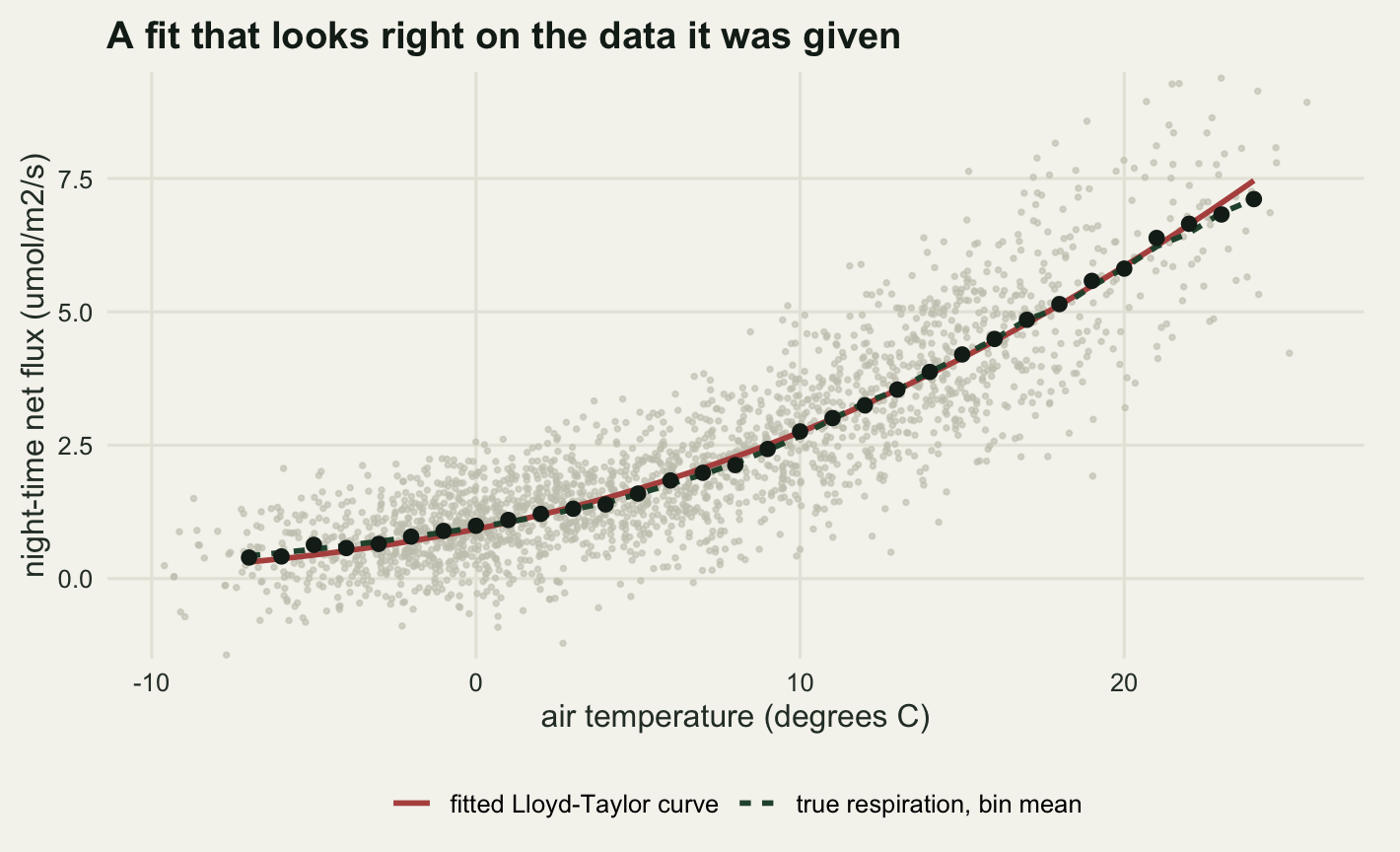
Given the assumption, the fit is ordinary nonlinear least squares on the night-time points with air temperature as the driver. Real processing chains usually prefer soil temperature; air temperature is used here because the simulation drove respiration with it, which removes a source of disagreement that would otherwise be confounded with the effect being measured.
dat_night <- data.frame(nee = nee_obs[night], tk = tk[night])
fit_nt <- nls(nee ~ rref * exp(e0 * (1 / (tref_k - t0_k) -
                                       1 / (tk - t0_k))),
              data = dat_night,
              start = list(rref = 2, e0 = 200))

co_nt <- summary(fit_nt)$coefficients
rref_hat <- unname(co_nt["rref", 1])
e0_hat <- unname(co_nt["e0", 1])
rref_se <- unname(co_nt["rref", 2])
e0_se <- unname(co_nt["e0", 2])

print(round(co_nt, 4))
Estimate Std. Error t value Pr(>|t|)
rref 2.7459 0.0117 234.1479 0
e0 280.0377 1.9788 141.5187 0print(round(c(rref_fitted = rref_hat, rref_true = rref_true,
rref_error_pct = 100 * (rref_hat / rref_true - 1),
rref_error_in_se = (rref_hat - rref_true) / rref_se), 3)) rref_fitted rref_true rref_error_pct rref_error_in_se
2.746 2.800 -1.931 -4.610 print(round(c(e0_fitted = e0_hat, e0_true = e0_true,
e0_error_pct = 100 * (e0_hat / e0_true - 1),
e0_error_in_se = (e0_hat - e0_true) / e0_se), 3)) e0_fitted e0_true e0_error_pct e0_error_in_se
280.038 208.000 34.634 36.405 The basal rate comes back at 2.746 umol/m2/s. The comparison printed beside it is not an accuracy check: 2.8 is a scale parameter, and the basal rate the night data actually saw is seasonal, rref_true * seas_r in the code above, running from 2.11 to 3.64 umol/m2/s through the year. A single annual estimate has no single truth to sit near. The temperature sensitivity comes back at 280 against a truth of 208, high by 34.63 per cent, with a standard error of 1.979. The estimate sits 36.4 standard errors from the value that generated the data.
That is not a failure of nls. It is the seasonal term in the truth doing exactly what seasonal terms do to a temperature response. Basal respiration is higher in July than in January for reasons that have nothing to do with the temperature of any given night: more foliage, more fine roots, more fresh litter. A single annual curve has to explain the summer nights being warm and the summer nights respiring more, and it charges both to temperature. The apparent temperature sensitivity of an annual fit is inflated, the confounding is between season and temperature rather than within either, and the standard error, computed as though the model were correct, says nothing about it.
Extrapolating into the day
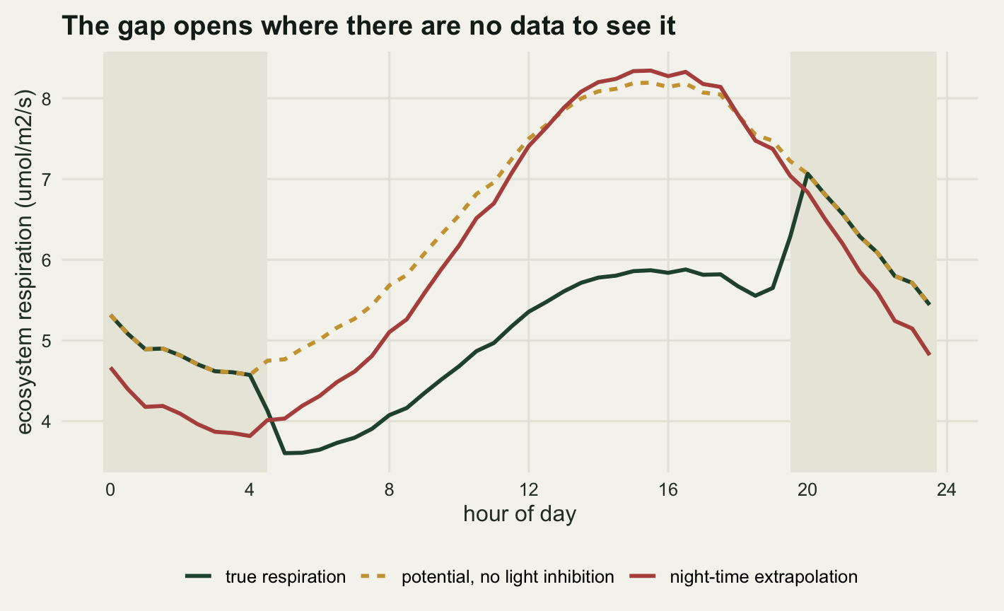
The fitted curve is now evaluated at every half hour of the year, including the ones in daylight where no respiration was ever observed, and gross primary production falls out of the definition. Since net exchange is respiration minus photosynthesis, photosynthesis is respiration minus net exchange.
reco_nt <- rref_hat * lt_shape(tk, e0_hat)
gpp_nt <- reco_nt - nee_obs

reco_nt_ann <- ann(reco_nt)
gpp_nt_ann <- ann(gpp_nt)
nee_nt_ann <- reco_nt_ann - gpp_nt_ann

err_reco_ann <- reco_nt_ann - reco_ann
err_gpp_ann <- gpp_nt_ann - gpp_ann
err_nee_ann <- nee_nt_ann - nee_ann

print(round(c(gpp_estimated = gpp_nt_ann, gpp_true = gpp_ann, gpp_error = err_gpp_ann,
              gpp_error_pct = 100 * err_gpp_ann / gpp_ann), 2))
gpp_estimated gpp_true gpp_error gpp_error_pct
1450.16 1297.22 152.95 11.79 print(round(c(reco_estimated = reco_nt_ann, reco_true = reco_ann, reco_error = err_reco_ann,
reco_error_pct = 100 * err_reco_ann / reco_ann), 2))reco_estimated reco_true reco_error reco_error_pct
1124.74 969.48 155.26 16.01 print(round(c(nee_estimated = nee_nt_ann, nee_true = nee_ann, nee_error = err_nee_ann,
nee_error_pct = 100 * err_nee_ann / abs(nee_ann)), 3))nee_estimated nee_true nee_error nee_error_pct
-325.423 -327.733 2.310 0.705 print(round(c(kok_cost = kok_ann, remainder = err_reco_ann - kok_ann,
kok_share_of_error_pct = 100 * kok_ann / err_reco_ann), 2)) kok_cost remainder kok_share_of_error_pct
116.34 38.92 74.93 Annual gross primary production comes out at 1450.2 gC/m2/yr against a truth of 1297.2, an overestimate of 152.9 gC/m2/yr or 11.79 per cent. Annual ecosystem respiration comes out at 1124.7 against 969.5, an overestimate of 155.3 gC/m2/yr or 16.01 per cent. Annual net ecosystem exchange comes out at -325.42 against -327.73, an error of 2.31 gC/m2/yr.
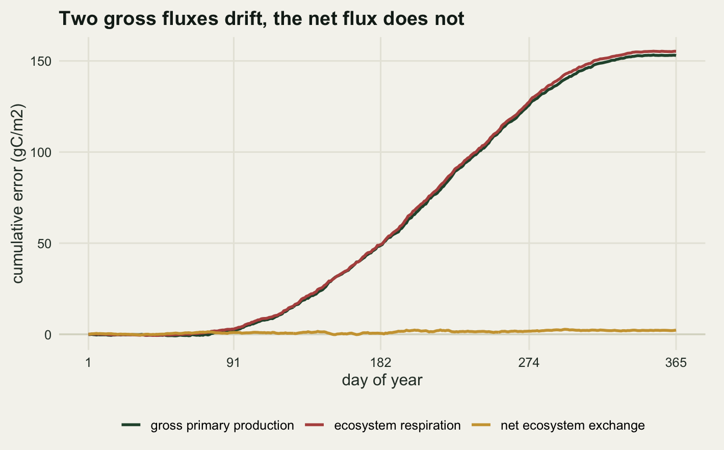
Two of those three lines are out by more than a hundred grams of carbon per square metre. The third is out by 2.31. That is the post.
The respiration error splits cleanly. Light inhibition of leaf respiration accounts for 116.3 gC/m2/yr of it, or 74.9 per cent, and the fitted annual curve sits above the potential respiration, the truth with the light inhibition switched off, by the remaining 38.9. The inflated temperature sensitivity is part of why that second gap is there rather than the whole of it: the sweep further down refits the basal rate at each assumed sensitivity, and an assumed value next to the truth still leaves most of that gap in place. Both push the same way, and neither is visible in the fit’s own diagnostics.
The two errors are one error
The reason annual net exchange survives is arithmetic rather than luck, and it is worth writing down. Let \(\hat{R}\) be the estimated respiration, \(R\) the true respiration, \(N\) the measured net flux and \(N^{*}\) the true net flux. The estimate of photosynthesis is \(\hat{G} = \hat{R} - N\) and the truth is \(G = R - N^{*}\), so
\[\hat{G} - G = (\hat{R} - R) - (N - N^{*})\]
The error in gross primary production is the error in respiration minus the measurement noise. Nothing else. Whatever the respiration model gets wrong is transferred into photosynthesis at a rate of one for one, with the same sign.
err_reco_hh <- reco_nt - reco_true
err_gpp_hh <- gpp_nt - gpp_true
noise_hh <- nee_obs - nee_true

identity_gap <- max(abs(err_gpp_hh - (err_reco_hh - noise_hh)))
cor_hh <- cor(err_reco_hh, err_gpp_hh)
slope_hh <- unname(coef(lm(err_gpp_hh ~ err_reco_hh))[2])
cor_pred <- sd(err_reco_hh) / sqrt(var(err_reco_hh) + var(noise_hh))

mon <- as.integer(cut(doy, breaks = c(0, cumsum(
  c(31, 28, 31, 30, 31, 30, 31, 31, 30, 31, 30, 31)))))
cor_day <- cor(tapply(err_reco_hh, doy, sum), tapply(err_gpp_hh, doy, sum))
cor_mon <- cor(tapply(err_reco_hh, mon, sum), tapply(err_gpp_hh, mon, sum))

print(c(identity_residual = formatC(identity_gap, format = "e", digits = 1)))
identity_residual
"2.7e-15" print(round(c(sd_model_error = sd(err_reco_hh), sd_noise = sd(noise_hh),
regression_slope = slope_hh), 4)) sd_model_error sd_noise regression_slope
0.7219 0.9853 0.9913 print(round(c(cor_half_hourly = cor_hh, cor_predicted = cor_pred,
cor_daily = cor_day, cor_monthly = cor_mon), 4))cor_half_hourly cor_predicted cor_daily cor_monthly
0.5877 0.5910 0.9431 0.9993 The identity holds to 2.7e-15, which is floating-point noise: the two errors are the same quantity offset by the measurement error, exactly, in every half hour of the year. The regression of one on the other has a slope of 0.9913.
Their correlation at half-hourly resolution is 0.5877, which is lower than the identity might suggest, and the second term is why. The model error has a standard deviation of 0.722 umol/m2/s against 0.985 for the noise, so the noise is the larger of the two at that resolution and dilutes the correlation to 0.591 on the standard formula, which is what came out. The noise is independent from one half hour to the next and the model error is not, so aggregating removes one and not the other: the correlation of daily sums is 0.9431 and of monthly sums 0.9993. At the timescale anyone reports a carbon flux, the two errors are the same number.
To separate what the noise does from what the model does, redraw the measurement error two hundred times over the same year and refit, holding the weather, the physiology and the true fluxes fixed.
n_rep <- 200
rep_out <- matrix(NA_real_, n_rep, 4)
for (b in seq_len(n_rep)) {
  set.seed(770000 + b)
  y_b <- nee_true + rnorm(n_hh, 0, sd_hh)
  fb <- nls(nee ~ rref * exp(e0 * (1 / (tref_k - t0_k) -
                                     1 / (tk - t0_k))),
            data = data.frame(nee = y_b[night], tk = tk[night]),
            start = list(rref = 2, e0 = 200))
  rc <- unname(coef(fb)[1]) * lt_shape(tk, unname(coef(fb)[2]))
  rep_out[b, ] <- c(ann(rc - reco_true), ann(rc - y_b - gpp_true),
                    ann(y_b - nee_true), unname(coef(fb)[2]))
}
colnames(rep_out) <- c("reco_err", "gpp_err", "nee_err", "e0")
rep_out <- as.data.frame(rep_out)

print(round(c(reco_err_mean = mean(rep_out$reco_err), reco_err_sd = sd(rep_out$reco_err),
              gpp_err_mean = mean(rep_out$gpp_err), gpp_err_sd = sd(rep_out$gpp_err)), 3))
reco_err_mean reco_err_sd gpp_err_mean gpp_err_sd
146.717 4.644 146.929 4.079 print(round(c(nee_err_mean = mean(rep_out$nee_err), nee_err_sd = sd(rep_out$nee_err),
gpp_err_min = min(rep_out$gpp_err),
nee_err_max_abs = max(abs(rep_out$nee_err))), 3)) nee_err_mean nee_err_sd gpp_err_min nee_err_max_abs
-0.212 2.860 136.766 7.219 print(round(c(e0_mean = mean(rep_out$e0), e0_sd = sd(rep_out$e0), e0_true = e0_true), 3))e0_mean e0_sd e0_true
280.686 2.320 208.000 Over 200 noise draws the annual respiration error averages 146.7 gC/m2/yr with a standard deviation of 4.64, and the annual photosynthesis error averages 146.9 with a standard deviation of 4.08. The annual net exchange error averages -0.212 with a standard deviation of 2.86, and its largest absolute value across all 200 draws is 7.22 gC/m2/yr. The smallest gross production error over the same draws is 136.8. The two distributions do not come close to overlapping, and they are not the same kind of quantity: one is measurement error, which averages down, and the other is model error, which does not. The year analysed above, with its respiration error of 155.3, sits towards the top of the replicate spread at 1.84 standard deviations above the mean, which is the extent of the luck involved. The fitted temperature sensitivity varies by 2.32 across draws around a mean of 280.7, so the noise is not what put it 72.7 above the truth either.
That figure is the argument for treating published net exchange and published gross production as different grades of evidence. A cross-site comparison of net exchange compares measurements. A cross-site comparison of gross production compares the outputs of a model that each site fitted separately, to its own night-time data, with its own seasonality and its own leaf physiology, and Wohlfahrt and Gu (2015) make the further point that the quantity those models produce is not even the same definition of photosynthesis that a leaf physiologist would use.
The daytime method, which does not extrapolate
The obvious response is to estimate daytime respiration from daytime data. That is what the light response method of Lasslop et al (2010) does: fit a rectangular hyperbola to the daytime net flux,
\[N = R_d - \frac{\alpha\, A_{\max}\, Q}{\alpha\, Q + A_{\max}}\]
with \(Q\) the photon flux, \(\alpha\) the initial quantum use efficiency, \(A_{\max}\) the saturating rate, and \(R_d\) an intercept that stands for daytime respiration. Because the intercept is estimated where the light inhibition is actually happening, it should see it. The catch is that \(R_d\) is the value of the curve at zero light, and there is very little daytime data near zero light, so the intercept is itself an extrapolation.
The fit is done in monthly windows, because a single annual light response curve would have the same seasonality problem as the annual temperature response.
rd_win <- rep(NA_real_, 12)
conv_win <- logical(12)
for (m in 1:12) {
  idx <- day_i[mon[day_i] == m]
  dd <- data.frame(nee = nee_obs[idx], ppfd = ppfd[idx])
  fm <- tryCatch(nls(nee ~ rd - a * am * ppfd / (a * ppfd + am),
                     data = dd, start = list(rd = 2, a = 0.04, am = 15),
                     algorithm = "port", lower = c(0, 0.001, 0.5),
                     upper = c(20, 0.3, 90)),
                 error = function(e) NULL)
  if (!is.null(fm)) {
    rd_win[m] <- unname(coef(fm)["rd"])
    conv_win[m] <- TRUE
  }
}

reco_dt <- reco_nt
reco_dt[day_i] <- rd_win[mon[day_i]]
gpp_dt <- reco_dt - nee_obs

gpp_dt_ann <- ann(gpp_dt)
reco_dt_ann <- ann(reco_dt)
mon_true <- as.vector(tapply(reco_true[day_i], mon[day_i], mean))
mon_nt <- as.vector(tapply(reco_nt[day_i], mon[day_i], mean))
rmse_nt <- sqrt(mean((mon_nt - mon_true)^2))
rmse_dt <- sqrt(mean((rd_win - mon_true)^2))
worst_m <- which.max(abs(rd_win / mon_true - 1))

low_cut <- 150
n_mon <- 12
low_i <- day_i[ppfd[day_i] < low_cut]
t_low <- mean(tair[low_i])
t_day <- mean(tair[day_i])
r_low <- mean(reco_true[low_i])
r_day <- mean(reco_true[day_i])

print(round(rbind(month = 1:12, truth = mon_true,
                  night_extrapolation = mon_nt, daytime_fit = rd_win), 3))
[,1] [,2] [,3] [,4] [,5] [,6] [,7] [,8] [,9]
month 1.000 2.000 3.000 4.000 5.000 6.000 7.000 8.000 9.000
truth 0.966 1.056 1.366 2.110 3.379 4.333 4.993 4.492 3.491
night_extrapolation 0.994 1.115 1.537 2.547 4.287 5.584 6.649 5.981 4.710
daytime_fit 0.463 1.164 1.353 2.466 3.309 3.712 5.086 4.018 3.084
[,10] [,11] [,12]
month 10.000 11.000 12.000
truth 2.529 1.687 1.140
night_extrapolation 3.385 2.072 1.241
daytime_fit 2.494 1.606 0.584print(round(c(gpp_daytime = gpp_dt_ann, gpp_error = gpp_dt_ann - gpp_ann,
reco_daytime = reco_dt_ann, reco_error = reco_dt_ann - reco_ann), 2)) gpp_daytime gpp_error reco_daytime reco_error
1263.24 -33.97 937.82 -31.66 print(round(c(monthly_rmse_night = rmse_nt, monthly_rmse_daytime = rmse_dt,
months_high_night = sum(mon_nt > mon_true), worst_month = worst_m,
months_high_daytime = sum(rd_win > mon_true),
windows_converged = sum(conv_win)), 3)) monthly_rmse_night monthly_rmse_daytime months_high_night
0.911 0.353 12.000
worst_month months_high_daytime windows_converged
1.000 3.000 12.000 print(round(c(mean_temp_low_light = t_low, mean_temp_all_daytime = t_day,
true_reco_low_light = r_low, true_reco_all_daytime = r_day), 3)) mean_temp_low_light mean_temp_all_daytime true_reco_low_light
8.705 11.935 2.434
true_reco_all_daytime
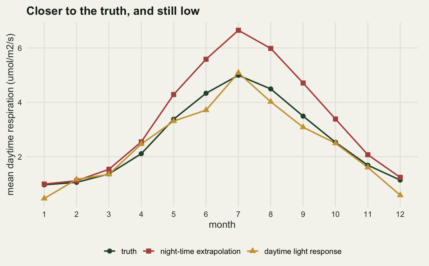
2.892 All 12 monthly windows converged. The daytime method returns an annual gross production of 1263.2 gC/m2/yr against a truth of 1297.2, an error of -33.97 gC/m2/yr, and an annual respiration of 937.8 against 969.5, an error of -31.66. Against the night-time method’s 152.9 gC/m2/yr that is a reduction of a factor of 4.5.
The monthly table says where the improvement comes from and what it costs. The night-time extrapolation is above the truth in all 12 months, by a margin that grows through the growing season: it is biased, consistently, in the direction the physiology predicts. The daytime fit is above the truth in only 3 months, and its monthly root mean squared error is 0.353 umol/m2/s against 0.911 for the extrapolation.
That is better, and it is still not unbiased. The daytime intercept sits below the truth in 9 of the 12 months, for a structural reason. The intercept is the value of the curve at zero light, so it is pinned by the half hours with least light, which are the ones near dawn and dusk, and those are also the cool ones: over daytime half hours below 150 umol/m2/s the mean air temperature is 8.71 degrees C against 11.93 for the daytime as a whole, and the true respiration in them averages 2.434 umol/m2/s against 2.892. A single constant intercept per month therefore reports a dawn-and-dusk respiration and gets used as a midday one. The published version of the method gives its intercept a temperature response for exactly this reason; the stripped-down version fitted here does not, and pays for it.
The worst month in relative terms is January, where the fitted intercept is 0.463 against a true 0.966: in a month with short days and almost no photosynthesis there is very little curvature in the light response for the fit to hold on to. The two methods are wrong in different ways, one with a bias that can be reasoned about from the physiology and the other with an anchoring problem that worsens as the light gets weaker, and neither is a measurement of daytime respiration.
What an assumed temperature sensitivity is worth
Processing chains commonly fix the temperature sensitivity rather than fit it, either at a literature value or at an estimate borrowed from a subset of the data, and then fit only the basal rate. That is defensible: the sensitivity is the badly determined parameter and holding it still stabilises everything else. It also means the published gross fluxes inherit whichever value was assumed.
With the sensitivity fixed, the model is linear in the basal rate, so no iteration is needed: the least squares estimate is a ratio of two sums over the night-time points.
e0_grid <- seq(100, 400, by = 25)
sens <- t(vapply(e0_grid, function(e0v) {
  gshape <- lt_shape(tk, e0v)
  rr <- sum(nee_obs[night] * gshape[night]) / sum(gshape[night]^2)
  rc <- rr * gshape
  gp <- rc - nee_obs
  c(e0 = e0v, rref = rr, gpp = ann(gp), reco = ann(rc),
    nee = ann(rc) - ann(gp))
}, numeric(5)))
sens <- as.data.frame(sens)

gpp_span <- max(sens$gpp) - min(sens$gpp)
nee_span <- max(sens$nee) - min(sens$nee)
gpp_low <- min(sens$gpp) - gpp_ann

print(round(sens, 2))
e0 rref gpp reco nee
1 100 2.83 1362.40 1036.97 -325.42
2 125 2.91 1392.16 1066.73 -325.42
3 150 2.95 1415.22 1089.80 -325.42
4 175 2.96 1432.07 1106.65 -325.42
5 200 2.94 1443.33 1117.91 -325.42
6 225 2.90 1449.73 1124.30 -325.42
7 250 2.84 1451.97 1126.55 -325.42
8 275 2.76 1450.77 1125.34 -325.42
9 300 2.67 1446.74 1121.32 -325.42
10 325 2.57 1440.46 1115.04 -325.42
11 350 2.46 1432.40 1106.98 -325.42
12 375 2.35 1422.96 1097.54 -325.42
13 400 2.23 1412.47 1087.05 -325.42print(round(c(gpp_span = gpp_span, gpp_span_pct = 100 * gpp_span / gpp_ann,
reco_span = max(sens$reco) - min(sens$reco), nee_span = nee_span), 3)) gpp_span gpp_span_pct reco_span nee_span
89.575 6.905 89.575 0.000 print(round(c(closest_gpp_to_truth = min(sens$gpp), truth = gpp_ann,
smallest_overestimate = gpp_low,
worst_overestimate = max(sens$gpp) - gpp_ann), 2)) closest_gpp_to_truth truth smallest_overestimate
1362.40 1297.22 65.18
worst_overestimate
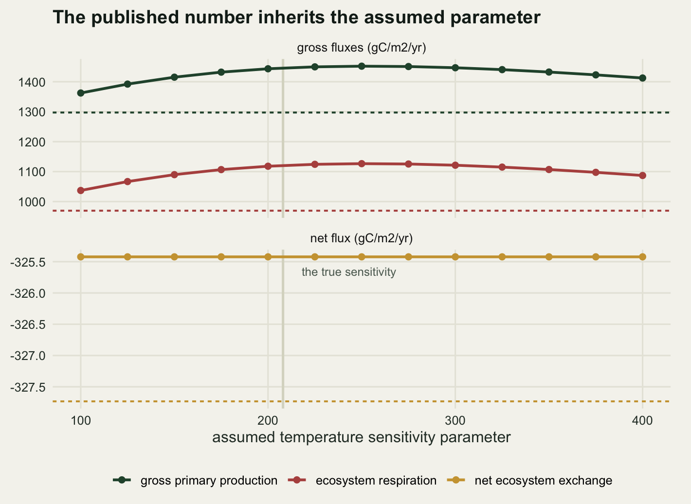
154.76 Across assumed sensitivities from 100 to 400, which spans the range that appears in the literature and comfortably contains the truth of 208, annual gross production moves from 1362.4 to 1452 gC/m2/yr, a span of 89.6 or 6.91 per cent of the true value. Annual respiration moves by 89.6 gC/m2/yr over the same range. Annual net exchange moves by 0.000000 gC/m2/yr, which is zero to numerical precision, because the identity from the previous section holds for any respiration model whatsoever.
The relationship is not monotone: gross production peaks at an assumed sensitivity in the middle of the range and falls away at both ends, because a very shallow response underestimates summer respiration while a very steep one, refitted, undershoots the basal rate. What matters more is where the truth sits relative to the whole curve. The closest any assumed value gets to the true annual gross production is 1362.4, still 65.2 gC/m2/yr too high. No choice of temperature sensitivity recovers the right answer, because the missing piece is not a temperature sensitivity: it is the light inhibition, which lives in a dimension this model does not have.
Letting the fit move through the season
The inflated temperature sensitivity came from asking one curve to cover a year in which the basal rate changed. The standard remedy is to stop asking: fit the relationship in short windows, so that within any one window the basal rate is close to constant and the only variation the fit has to explain is the night-to-night weather. Here the window is a fortnight, which is the sort of length used in practice.
win_len <- 14
wid <- pmin(((doy - 1) %/% win_len) + 1, 26)
n_win <- max(wid)
e0_w <- rep(NA_real_, n_win)
rref_w <- rep(NA_real_, n_win)

for (w in seq_len(n_win)) {
  ii <- which(night & wid == w)
  fw <- tryCatch(nls(y ~ rr * exp(ee * (1 / (tref_k - t0_k) -
                                          1 / (x - t0_k))),
                     data = data.frame(y = nee_obs[ii], x = tk[ii]),
                     start = list(rr = 2, ee = 200), algorithm = "port",
                     lower = c(0.01, 0), upper = c(30, 1000)),
                 error = function(e) NULL)
  if (!is.null(fw)) {
    rref_w[w] <- unname(coef(fw)[1])
    e0_w[w] <- unname(coef(fw)[2])
  }
}

reco_sw <- rref_w[wid] * lt_shape(tk, e0_w[wid])
gpp_sw <- reco_sw - nee_obs
rref_w_true <- as.vector(tapply(rref_true * seas_r, wid, mean))

reco_sw_ann <- ann(reco_sw)
gpp_sw_ann <- ann(gpp_sw)
pot_ann <- ann(reco_pot)

rref_cor <- cor(rref_w, rref_w_true)
rref_rmse <- sqrt(mean((rref_w - rref_w_true)^2))

print(round(c(windows = n_win, converged = sum(!is.na(e0_w)), e0_mean = mean(e0_w),
              e0_sd = sd(e0_w), e0_true = e0_true, e0_annual_fit = e0_hat,
              rref_correlation = rref_cor, rref_rmse = rref_rmse), 3))
windows converged e0_mean e0_sd
26.000 26.000 213.501 19.273
e0_true e0_annual_fit rref_correlation rref_rmse
208.000 280.038 0.979 0.113 print(round(c(reco_short_window = reco_sw_ann, reco_error = reco_sw_ann - reco_ann,
reco_error_annual_fit = err_reco_ann,
recovered = err_reco_ann - (reco_sw_ann - reco_ann)), 2)) reco_short_window reco_error reco_error_annual_fit
1098.56 129.07 155.26
recovered
26.19 print(round(c(gpp_short_window = gpp_sw_ann, gpp_error = gpp_sw_ann - gpp_ann,
potential_reco = pot_ann, error_against_potential = reco_sw_ann - pot_ann,
error_against_potential_pct =
100 * (reco_sw_ann - pot_ann) / pot_ann), 2)) gpp_short_window gpp_error
1423.98 126.76
potential_reco error_against_potential
1085.82 12.74
error_against_potential_pct
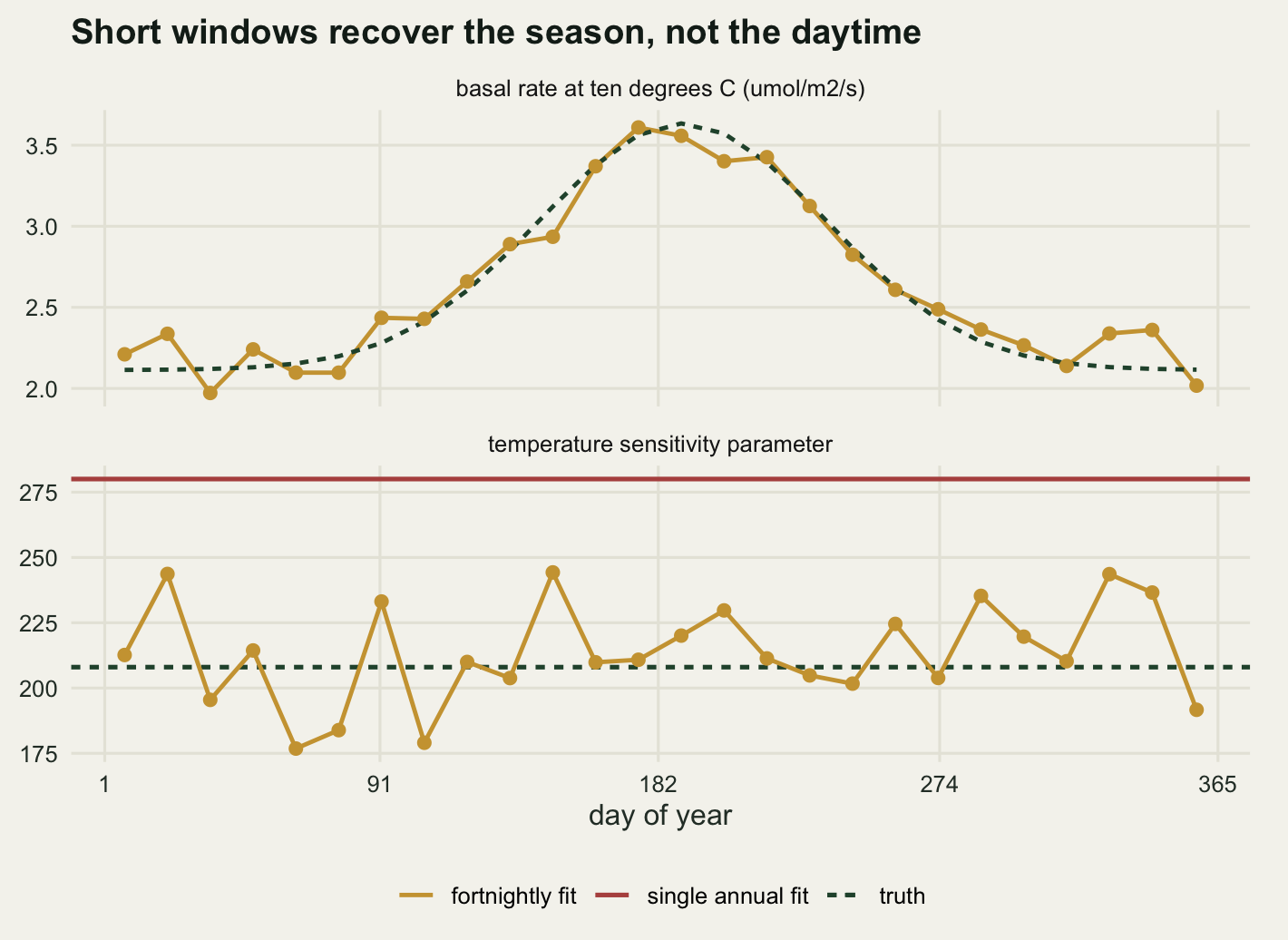
1.17 All 26 fortnightly windows converged. The mean fitted sensitivity is 213.5 against a truth of 208, with a standard deviation across windows of 19.3. The annual fit gave 280. That is the whole of the seasonal confounding removed by nothing more than shortening the window, and it is the clearest illustration on this page of what a temperature response fitted across a season actually measures. The fortnightly basal rates track the true seasonal cycle with a correlation of 0.979 and a root mean squared error of 0.113 umol/m2/s.
The annual totals move accordingly, and then stop moving. Short-window respiration comes out at 1098.6 gC/m2/yr against a truth of 969.5, an error of 129.1, where the annual fit had an error of 155.3. The flexibility bought back 26.2 gC/m2/yr and left 129.1 on the table.
The residue is not a coincidence. The potential respiration in the truth, the value the temperature would give with no light inhibition at all, totals 1085.8 gC/m2/yr, and the short-window estimate lands 12.7 gC/m2/yr from it, 1.17 per cent. The fortnightly fit has recovered the respiration the ecosystem would have had if the leaves had gone on respiring in the light at their night-time rate. That is the correct answer to the question the night-time data can answer, and it is not the question that was asked. Flexibility fixes the part of the error that comes from a non-stationary temperature response and cannot touch the part that comes from extrapolating night physiology into daylight, because no amount of night-time data contains any information about what the leaves do once the sun is up.
The honest limit
The truth column is a simulation, and that is the only reason any of the errors above could be quoted as numbers. In the field nobody knows gross primary production: no instrument, no calibration standard, no independent series to check a partitioning against, which is why the argument in the literature is conducted between methods rather than against a reference. Desai et al (2008) ran twenty-three partitioning methods over ten site-years of temperate forest and found most of them within ten per cent of each other on annual gross production and annual respiration. Ten per cent is the same order as the bias measured here, and a gap that size between two sites would ordinarily be given an ecological reading.
The size of the light inhibition is assumed. Wehr et al (2016) measured it at ecosystem scale with isotopic partitioning at one temperate forest and reported daytime respiration well below the night-time extrapolation through the growing season, but the magnitude varies with species, nutrition and season, and it is not something a processing chain can read off its own data. A different assumption would change the size of the bias while leaving the structure of the argument alone, and the structure is what transfers: an error in modelled respiration goes into gross production one for one.
Three parts of the measurement chain declared out of scope all feed back into this fit. The friction velocity filter removes the calmest nights, which are also the coldest and the ones that would anchor the low-temperature end of the response, so the filter and the fitted sensitivity are not independent (Papale et al 2006). Carbon dioxide stored in the canopy air below the sensor is released at dawn and shows up in the night-time data if it is not accounted for. Advection down a slope removes respired carbon the tower never sees, and the loss is largest on exactly the calm nights the filter is trying to salvage. Baldocchi (2003) puts the resulting uncertainty on an annual net exchange from a good site at well over a hundred grams of carbon per square metre, which is the same order as everything measured above, and it applies to the net flux that came out clean here.
Two smaller things: the daytime method was given the correct functional form for the light response, which no real analysis is, and the fortnightly windows were fitted to a year with no gaps, whereas a real year loses a large share of its night-time points to the friction velocity filter before any of this starts.
Where to go next
What these gross fluxes do to an annual carbon budget, once they are added up and compared with something measured on the ground, is checking an annual flux budget. If the nonlinear fitting is the unfamiliar part rather than the ecology, the mechanics of nls and its starting values are set out in nonlinear regression in R with nls.
There is a version of this exercise worth running on your own tower data before publishing a gross flux from it: fit the night-time response on short windows, fit it on the whole year, fix the sensitivity at the two ends of the plausible range, and report the spread of annual gross production across those choices next to the number itself. The spread here was 89.6 gC/m2/yr from the fixed-sensitivity sweep alone. A gross production quoted without it is quoting a model output as a measurement.
References
Lloyd J, Taylor JA 1994 Functional Ecology 8(3):315-323 (10.2307/2389824)
Reichstein M, et al 2005 Global Change Biology 11(9):1424-1439 (10.1111/j.1365-2486.2005.001002.x)
Lasslop G, Reichstein M, Papale D, Richardson AD, Arneth A, Barr A, Stoy P, Wohlfahrt G 2010 Global Change Biology 16(1):187-208 (10.1111/j.1365-2486.2009.02041.x)
Wohlfahrt G, Gu L 2015 Plant, Cell and Environment 38(12):2500-2507 (10.1111/pce.12569)
Wehr R, Munger JW, McManus JB, Nelson DD, Zahniser MS, Davidson EA, Wofsy SC, Saleska SR 2016 Nature 534(7609):680-683 (10.1038/nature17966)
Desai AR, et al 2008 Agricultural and Forest Meteorology 148(6-7):821-838 (10.1016/j.agrformet.2007.11.012)
Papale D, et al 2006 Biogeosciences 3(4):571-583 (10.5194/bg-3-571-2006)
Baldocchi DD 2003 Global Change Biology 9(4):479-492 (10.1046/j.1365-2486.2003.00629.x)