library(ggplot2)

te_pal <- list(forest = "#275139", green = "#2f8f63", sage = "#93a87f",
               clay = "#b5534e", gold = "#cda23f", line = "#dad9ca",
               ink = "#16241d", paper = "#f5f4ee")

theme_te <- function() {
  theme_minimal(base_size = 12) +
    theme(panel.grid.minor = element_blank(),
          panel.grid.major = element_line(colour = "#e7e6dc"),
          plot.background = element_rect(fill = "#f5f4ee", colour = NA),
          panel.background = element_rect(fill = "#f5f4ee", colour = NA),
          plot.title = element_text(face = "bold", colour = te_pal$ink),
          axis.title = element_text(colour = te_pal$ink),
          legend.position = "bottom")
}

f2 <- function(x) sprintf("%.2f", x)
f3 <- function(x) sprintf("%.3f", x)
f4 <- function(x) sprintf("%.4f", x)The recalcitrant pool and the asymptote
R
decomposition
nonlinear regression
ecology tutorial
ggplot2
Two-pool and asymptotic decay models fit the same litterbag data and disagree about the limit value: likelihood profiles, AIC power and harvest design in R.
The litterbags go out in October. Four hundred of them, ten grams of oven-dried leaf litter each, pinned flat on the forest floor in blocks, and the schedule on the back of the field notebook says when they come back: three months, six months, nine months, a year, then eighteen months, two years, three years. Four bags per harvest per treatment, washed, dried, weighed, ash-corrected. By the end of the second year the mass-remaining curve has stopped doing anything interesting. The points at two years and three years sit on top of each other, and the obvious reading of that is that the litter has reached a floor.
That reading has a name and a parameter. The asymptotic model writes mass remaining as \(M(t) = A + (1 - A)e^{-kt}\), and \(A\) is the limit value of decomposition: the fraction of the original litter that the model says never goes. Limit values get reported, compared across species, regressed on lignin and on nitrogen, and fed into soil carbon models as the input that stabilises. There is a second model that produces the same flattening without any such claim. The two-pool double exponential writes \(M(t) = ae^{-k_1t} + (1 - a)e^{-k_2t}\): a fast pool of solubles and cellulose leaving at rate \(k_1\), a slow lignified residue leaving at rate \(k_2\), and if \(k_2\) is small enough the curve flattens over a three-year study while every gram of it still decomposes eventually.
The two models make incompatible statements about what happens after the study ends and nearly identical statements about what happens during it. That is the subject here. The post fits both to litterbag data, profiles the likelihood, measures how often the model comparison can tell them apart, and then measures what the harvest schedule does to all of it.
The data are simulated, and the reason is that a limit value cannot be checked against reality inside a human career: a simulated litterbag study comes with a truth column that says whether the slow pool decomposes or not. Fitting these curves as a routine job, with the residual checks and the ash correction, is covered separately in fitting litter decomposition curves; this post assumes the fit works and asks what the fitted parameter means.
Three models and how they nest
All three models are written on the same scale: mass remaining as a proportion of the mass that went into the bag, starting at one. The single exponential is Olson’s, and it has one rate. The two-pool model splits the litter into a fraction \(a\) that leaves fast and a fraction \(1 - a\) that leaves slowly. The asymptotic model keeps a fraction \(A\) back permanently.
The nesting is worth stating before any fitting, because it decides what a comparison between them can mean. The asymptotic model is the two-pool model with \(k_2\) set to zero, with \(A = 1 - a\) and \(k = k_1\). The single exponential is the two-pool model with \(a = 1\), and it is also the asymptotic model with \(A = 0\). So the three are one family, and the interesting boundary is \(k_2 = 0\): a permanent limit value is not a different theory of decomposition, it is the edge of the parameter space of the two-pool model.
m_single <- function(t, k) exp(-k * t)
m_two <- function(t, a, k1, k2) a * exp(-k1 * t) + (1 - a) * exp(-k2 * t)
m_asym <- function(t, A, k) A + (1 - A) * exp(-k * t)

tcheck <- c(0.5, 2, 10, 40)
nest <- rbind(years = tcheck,
              two_pool_with_k2_at_zero = m_two(tcheck, 0.55, 3.5, 0),
              asymptotic_with_A_at_one_minus_a = m_asym(tcheck, 0.45, 3.5),
              two_pool_with_a_at_one = m_two(tcheck, 1, 3.5, 0.08),
              single_exponential = m_single(tcheck, 3.5))
print(round(nest, 6))
[,1] [,2] [,3] [,4]
years 0.500000 2.000000 10.00 40.00
two_pool_with_k2_at_zero 0.545576 0.450502 0.45 0.45
asymptotic_with_A_at_one_minus_a 0.545576 0.450502 0.45 0.45
two_pool_with_a_at_one 0.173774 0.000912 0.00 0.00
single_exponential 0.173774 0.000912 0.00 0.00round(c(largest_gap_to_the_asymptotic_model = max(abs(nest[2, ] - nest[3, ])),
largest_gap_to_the_single_exponential = max(abs(nest[4, ] - nest[5, ]))), 8) largest_gap_to_the_asymptotic_model largest_gap_to_the_single_exponential
0 0 The two lines of arithmetic confirm the algebra: with \(k_2\) at zero the two-pool model returns the asymptotic model to the last decimal place the machine keeps, and with \(a\) at one it returns the single exponential. Nothing in the rest of the post depends on that check, but a model comparison between two forms that turn out not to nest the way you thought is a comparison of nothing, and the check costs one chunk.
The simulated study follows the schedule in the notebook: seven harvests at three months, six months, nine months, one year, eighteen months, two years and three years, with four bags at each. The generating process is a two-pool decay with a fast fraction of 0.55 leaving at 3.5 per year (half of it gone in ten weeks) and a slow fraction leaving at 0.08 per year, a half-life of about nine years. Nothing in that process has a limit value. Every gram decomposes; the slow half is simply slow. Measurement error on the recovered mass is added as a normal deviate with a standard deviation of 0.03 of the initial mass, which is what bag-to-bag variation in a careful study looks like once the roots and the soil have been picked off.
set.seed(20260726)

a_true <- 0.55
k1_true <- 3.5
k2_true <- 0.08
sd_true <- 0.03
n_bag <- 4
harvest <- c(0.25, 0.5, 0.75, 1, 1.5, 2, 3)

tt <- rep(harvest, each = n_bag)
yy <- m_two(tt, a_true, k1_true, k2_true) + rnorm(length(tt), 0, sd_true)
n_obs <- length(yy)
mbar <- tapply(yy, tt, mean)

print(round(rbind(harvest_years = harvest,
                  mean_mass_remaining = as.numeric(mbar),
                  true_mass_remaining = m_two(harvest, a_true, k1_true, k2_true)), 4))
[,1] [,2] [,3] [,4] [,5] [,6] [,7]
harvest_years 0.2500 0.5000 0.7500 1.0000 1.5000 2.0000 3.0000
mean_mass_remaining 0.6695 0.5592 0.4829 0.4025 0.3996 0.3563 0.3546
true_mass_remaining 0.6704 0.5279 0.4636 0.4320 0.4020 0.3840 0.3540round(c(bags = n_obs, harvests = length(harvest), bags_per_harvest = n_bag,
true_mass_left_at_10_years = m_two(10, a_true, k1_true, k2_true),
true_mass_left_at_30_years = m_two(30, a_true, k1_true, k2_true),
true_mass_left_at_100_years = m_two(100, a_true, k1_true, k2_true),
slow_pool_half_life_years = log(2) / k2_true,
fast_pool_half_life_years = log(2) / k1_true), 4) bags harvests
28.0000 7.0000
bags_per_harvest true_mass_left_at_10_years
4.0000 0.2022
true_mass_left_at_30_years true_mass_left_at_100_years
0.0408 0.0002
slow_pool_half_life_years fast_pool_half_life_years
8.6643 0.1980 Twenty-eight bags. The mean at two years is 0.3563 and at three years 0.3546, a drop of 0.0016 over a year, which is the flattening that starts the argument. The truth behind those two numbers is a decline from 0.3840 to 0.3540, and it keeps going: 0.2022 at ten years, 0.0408 at thirty and 0.0002 at a century. The floor in the data is not a floor.
Fitting all three
Starting values are the part of nonlinear fitting that goes wrong first, and the general treatment is in starting values and identifiability. For these three models the values can be read off the data with no optimisation at all. The fast rate comes from the first harvest, treating the early loss as if it were a single exponential. The slow rate comes from a straight line through the logged means of the last three harvests. The fast fraction is one minus the mean at the final harvest, and the limit value starts at that final mean.
start_values <- function(t, y) {
  m <- tapply(y, t, mean)
  tu <- as.numeric(names(m))
  last3 <- seq(length(m) - 2, length(m))
  k2 <- max(0.01, -unname(coef(lm(log(as.numeric(m[last3])) ~ tu[last3]))[2]))
  k1 <- max(0.5, -log(as.numeric(m[1])) / tu[1])
  c(a = min(0.9, max(0.1, 1 - as.numeric(m[length(m)]))), k1 = k1, k2 = k2,
    A = as.numeric(m[length(m)]))
}
st <- start_values(tt, yy)
print(round(st, 4))
a k1 k2 A
0.6454 1.6052 0.0689 0.3546 With those in hand nls fits all three without complaint. nls minimises the residual sum of squares, which for normal errors of constant variance is the maximum likelihood fit, so the AIC that stats::AIC returns is the Gaussian one and can be computed by hand from the residual sum of squares as a check.
d <- data.frame(t = tt, y = yy)

fit_1 <- nls(y ~ exp(-k * t), data = d, start = list(k = st["k1"]))
fit_2 <- nls(y ~ a * exp(-k1 * t) + (1 - a) * exp(-k2 * t), data = d,
             start = list(a = st["a"], k1 = st["k1"], k2 = st["k2"]))
fit_A <- nls(y ~ A + (1 - A) * exp(-k * t), data = d,
             start = list(A = st["A"], k = st["k1"]))

rss_of <- function(fit) sum(residuals(fit)^2)
aic_by_hand <- function(rss, n, p) n * log(2 * pi * rss / n) + n + 2 * (p + 1)

print(round(coef(fit_1), 4))
k
0.7174 print(round(coef(fit_2), 4)) a k1 k2
0.5794 2.9470 0.0637 print(round(coef(fit_A), 4)) A k
0.3653 2.5396 tab <- rbind(
`single exponential` = c(np = 1, rss = rss_of(fit_1), aic = AIC(fit_1),
by_hand = aic_by_hand(rss_of(fit_1), n_obs, 1)),
`two pool` = c(np = 3, rss = rss_of(fit_2), aic = AIC(fit_2),
by_hand = aic_by_hand(rss_of(fit_2), n_obs, 3)),
`asymptotic` = c(np = 2, rss = rss_of(fit_A), aic = AIC(fit_A),
by_hand = aic_by_hand(rss_of(fit_A), n_obs, 2)))
tab <- cbind(tab, delta_aic = tab[, "aic"] - min(tab[, "aic"]))
print(round(tab, 4)) np rss aic by_hand delta_aic
single exponential 1 0.5777 -25.2039 -25.2039 78.1361
two pool 3 0.0307 -103.3400 -103.3400 0.0000
asymptotic 2 0.0331 -103.2551 -103.2551 0.0849The single exponential is out of the argument: its residual sum of squares is 0.5777 against 0.0307 for the two-pool model, and it sits 78.14 AIC units above it. The flattening is real and one rate cannot produce it. The hand-computed AIC agrees with stats::AIC to four decimal places, which is the check that the likelihood being profiled later is the same likelihood nls maximised.
The other two are not out of the argument. The two-pool fit puts 0.5794 of the mass in a fast pool leaving at 2.9470 per year and the rest in a slow pool at 0.0637 per year, against a truth of 0.55, 3.5 and 0.08: close on the fraction, low on the fast rate, low on the slow rate. The asymptotic fit puts 0.3653 of the mass beyond reach for ever and decays the rest at 2.5396 per year. The gap between them is 0.0849 AIC units. On the usual reading of AIC differences that is no evidence at all, and the two models say different things about every year after the last harvest.
tg_in <- seq(0, 3, length.out = 200)
tg_out <- seq(0, 30, length.out = 400)

curve_frame <- function(tg, panel) {
  data.frame(
    t = rep(tg, 4),
    m = c(m_two(tg, a_true, k1_true, k2_true),
          m_single(tg, coef(fit_1)["k"]),
          m_two(tg, coef(fit_2)["a"], coef(fit_2)["k1"], coef(fit_2)["k2"]),
          m_asym(tg, coef(fit_A)["A"], coef(fit_A)["k"])),
    model = factor(rep(c("Truth (two pool)", "Single exponential",
                         "Two pool fit", "Asymptotic fit"), each = length(tg)),
                   levels = c("Truth (two pool)", "Single exponential",
                              "Two pool fit", "Asymptotic fit")),
    panel = panel)
}
cf <- rbind(curve_frame(tg_in, "Inside the study: 0 to 3 years"),
            curve_frame(tg_out, "Extrapolated: 0 to 30 years"))
cf$panel <- factor(cf$panel, levels = c("Inside the study: 0 to 3 years",
                                        "Extrapolated: 0 to 30 years"))
pts <- data.frame(t = tt, y = yy, panel = factor("Inside the study: 0 to 3 years",
                                                 levels = levels(cf$panel)))

ggplot(cf, aes(t, m, colour = model, linetype = model)) +
  # pale sage put the data behind three full-strength curves, so the eye landed
  # on the single exponential before it found the bags: the points carry the
  # same forest as the thumbnail, which is darker than any of the three fits
  geom_point(data = pts, aes(t, y), inherit.aes = FALSE, size = 1.9,
             colour = te_pal$forest, alpha = 0.9) +
  geom_line(linewidth = 0.9) +
  facet_wrap(~panel, scales = "free_x") +
  scale_colour_manual(values = c(te_pal$ink, te_pal$gold, te_pal$green,
                                 te_pal$clay), name = NULL) +
  scale_linetype_manual(values = c(2, 1, 1, 4), name = NULL) +
  scale_y_continuous(limits = c(0, 1)) +
  labs(x = "Years since the bags went out", y = "Mass remaining",
       title = "Same data, same fit, two different futures") +
  theme_te() +
  theme(strip.text = element_text(colour = te_pal$ink, face = "bold", size = 9),
        plot.margin = margin(6, 12, 6, 6))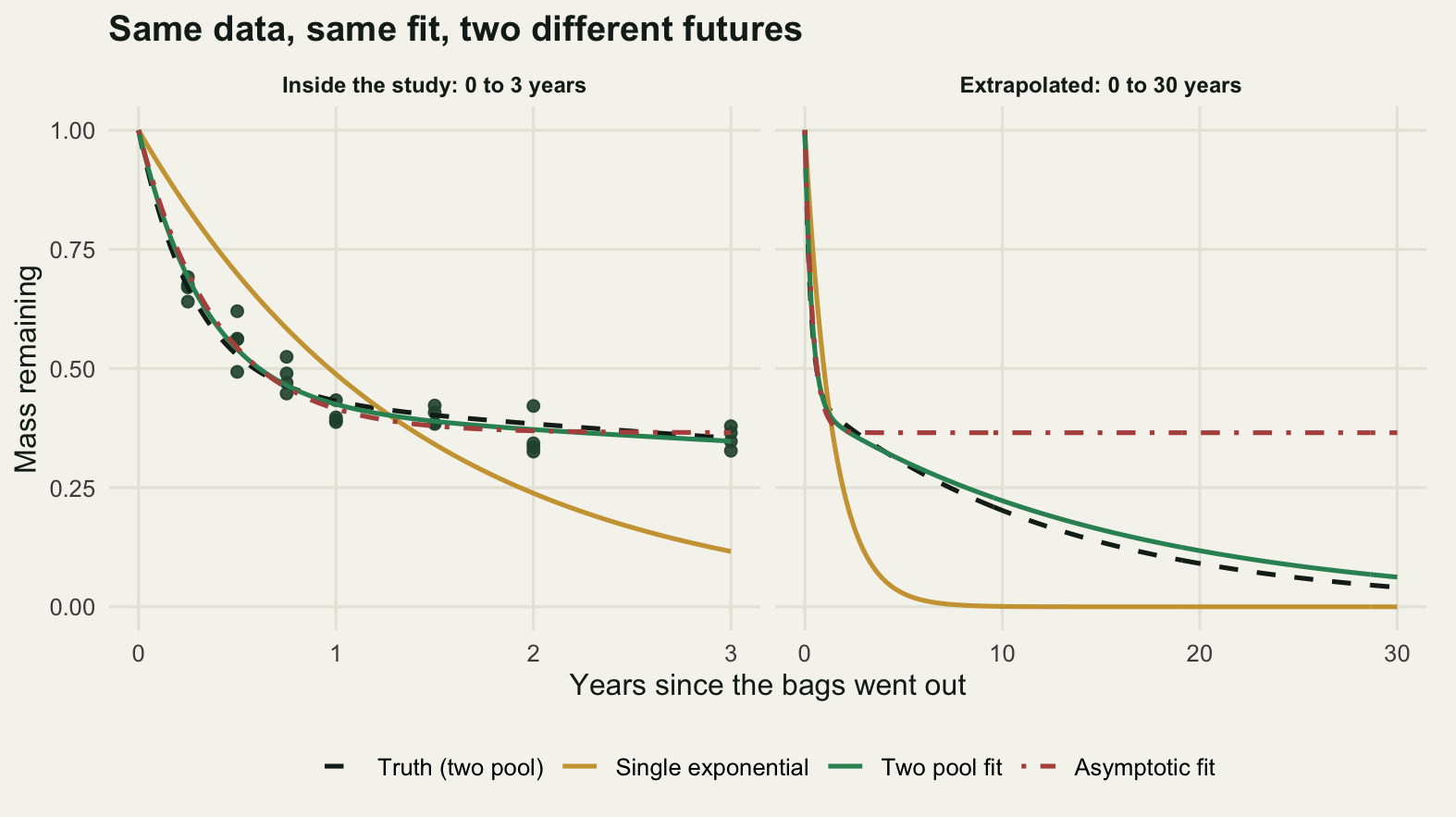
cf2 <- unname(coef(fit_2))
cfA <- unname(coef(fit_A))
two_pool_at <- function(t) m_two(t, cf2[1], cf2[2], cf2[3])
asym_at <- function(t) m_asym(t, cfA[1], cfA[2])

tg <- seq(0, 3, length.out = 601)
gap <- abs(two_pool_at(tg) - asym_at(tg))
gap30 <- abs(two_pool_at(30) - asym_at(30))

round(c(largest_gap_inside_the_study = max(gap),
        gap_at_the_last_harvest = gap[tg == 3],
        measurement_sd = sd_true,
        gap_in_units_of_the_measurement_sd = max(gap) / sd_true,
        gap_at_30_years = gap30,
        gap_at_30_relative_to_inside = gap30 / max(gap),
        two_pool_prediction_at_30_years = two_pool_at(30),
        asymptotic_prediction_at_30_years = asym_at(30),
        truth_at_30_years = m_two(30, a_true, k1_true, k2_true)), 4)
largest_gap_inside_the_study gap_at_the_last_harvest
0.0180 0.0180
measurement_sd gap_in_units_of_the_measurement_sd
0.0300 0.6015
gap_at_30_years gap_at_30_relative_to_inside
0.3030 16.7926
two_pool_prediction_at_30_years asymptotic_prediction_at_30_years
0.0623 0.3653
truth_at_30_years
0.0408 Over the three years the study covers, the largest distance between the two fitted curves is 0.0180 of the initial mass, which is 0.60 times the measurement standard deviation on one bag and would need a much larger study to see. At thirty years the same two curves are 0.3030 apart, 16.79 times the largest gap inside the study. The models are separated almost entirely in the region where there are no data.
The profile, and the end that sits on the boundary
The standard error nls prints for \(k_2\) comes from a quadratic approximation to the likelihood surface at the optimum. Near a boundary that approximation is worth little, and \(k_2 = 0\) is exactly where the interesting hypothesis lives. The honest tool is the likelihood profile: fix the parameter at each of a grid of values, re-optimise everything else, and keep the interval of values that stay within 1.92 log-likelihood units of the maximum, which is the conventional two-unit rule of thumb sharpened to the chi-squared quantile it approximates.
Profiling needs a fitter that can sit on the boundary, and nls cannot: at \(k_2 = 0\) the two-pool model loses a parameter and the Gauss-Newton step becomes singular. So the profile and every simulation from here on uses optim on the residual sum of squares, with the fraction on a logit scale and the rates on a log scale so that neither can wander out of its range. The fit is run twice from the point the first run reached, which is the cheapest guard there is against Nelder-Mead stopping early.
expit <- function(z) 1 / (1 + exp(-z))
logit <- function(p) log(p / (1 - p))

fit_two_pool <- function(t, y, start) {
  f <- function(z) sum((y - m_two(t, expit(z[1]), exp(z[2]), exp(z[3])))^2)
  z <- unname(c(logit(start["a"]), log(start["k1"]), log(start["k2"])))
  for (i in 1:2) z <- optim(z, f, control = list(reltol = 1e-12, maxit = 3000))$par
  a <- expit(z[1]); k1 <- exp(z[2]); k2 <- exp(z[3])
  if (k2 > k1) { a <- 1 - a; s <- k1; k1 <- k2; k2 <- s }
  list(par = c(a = a, k1 = k1, k2 = k2), rss = f(z))
}

fit_asymptote <- function(t, y, start) {
  f <- function(z) sum((y - m_asym(t, expit(z[1]), exp(z[2])))^2)
  z <- unname(c(logit(start["A"]), log(start["k1"])))
  for (i in 1:2) z <- optim(z, f, control = list(reltol = 1e-12, maxit = 3000))$par
  list(par = c(A = expit(z[1]), k = exp(z[2])), rss = f(z))
}

loglik <- function(rss, n) -n / 2 * (log(2 * pi * rss / n) + 1)
thr <- qchisq(0.95, 1) / 2

check <- fit_two_pool(tt, yy, st)
round(c(optim_a = check$par["a"], nls_a = coef(fit_2)["a"],
        optim_k1 = check$par["k1"], nls_k1 = coef(fit_2)["k1"],
        optim_k2 = check$par["k2"], nls_k2 = coef(fit_2)["k2"],
        optim_rss = check$rss, nls_rss = rss_of(fit_2),
        log_likelihood_threshold = thr), 5)
optim_a.a nls_a.a optim_k1.k1
0.57939 0.57939 2.94696
nls_k1.k1 optim_k2.k2 nls_k2.k2
2.94695 0.06368 0.06368
optim_rss nls_rss log_likelihood_threshold
0.03074 0.03074 1.92073 The optim fit reproduces the nls fit to four decimal places, so the two machineries are fitting the same model and the profile below is a profile of the likelihood that produced the AIC table above.
profile_k <- function(t, y, which, grid, start) {
  sapply(grid, function(v) {
    if (which == "k2") {
      f <- function(z) sum((y - m_two(t, expit(z[1]), exp(z[2]), v))^2)
      z <- unname(c(logit(0.6), log(max(start["k1"], 0.5))))
    } else {
      f <- function(z) sum((y - m_two(t, expit(z[1]), v, exp(z[2])))^2)
      z <- unname(c(logit(0.6), log(max(start["k2"], 0.01))))
    }
    for (i in 1:2) z <- optim(z, f, control = list(reltol = 1e-12, maxit = 3000))$par
    f(z)
  })
}

profile_A <- function(t, y, grid, k0) {
  sapply(grid, function(v) {
    optim(log(k0), function(z) sum((y - m_asym(t, v, exp(z)))^2),
          method = "Brent", lower = -6, upper = 5)$value
  })
}

interval_of <- function(grid, rss, n) {
  ll <- loglik(rss, n)
  keep <- ll >= max(ll) - thr
  c(lo = min(grid[keep]), hi = max(grid[keep]))
}

g_k2 <- seq(0, 0.6, by = 0.002)
g_k1 <- seq(1.5, 9, by = 0.01)
g_A <- seq(0, 0.55, by = 0.002)

pr_k2 <- profile_k(tt, yy, "k2", g_k2, st)
pr_k1 <- profile_k(tt, yy, "k1", g_k1, st)
pr_A <- profile_A(tt, yy, g_A, coef(fit_A)["k"])

ci_k2 <- unname(interval_of(g_k2, pr_k2, n_obs))
ci_k1 <- unname(interval_of(g_k1, pr_k1, n_obs))
ci_A <- unname(interval_of(g_A, pr_A, n_obs))

round(c(k2_lower = ci_k2[1], k2_upper = ci_k2[2],
        k2_width = ci_k2[2] - ci_k2[1], k2_estimate = cf2[3], k2_truth = k2_true,
        slowest_half_life_in_the_interval = log(2) / ci_k2[2],
        k1_lower = ci_k1[1], k1_upper = ci_k1[2],
        k1_width = ci_k1[2] - ci_k1[1],
        A_lower = ci_A[1], A_upper = ci_A[2],
        A_width = ci_A[2] - ci_A[1],
        A_width_as_percent_either_side = 100 * (ci_A[2] - ci_A[1]) / 2), 4)
k2_lower k2_upper
0.0000 0.1400
k2_width k2_estimate
0.1400 0.0637
k2_truth slowest_half_life_in_the_interval
0.0800 4.9511
k1_lower k1_upper
2.3400 3.8300
k1_width A_lower
1.4900 0.3440
A_upper A_width
0.3860 0.0420
A_width_as_percent_either_side
2.1000 The interval for the slow rate runs from 0.0000 to 0.1400 per year. Its lower end is the boundary. Every value between zero and 0.1400 is inside 1.92 log-likelihood units of the best fit, and zero is the asymptotic model, so the study cannot distinguish litter that stops decomposing from litter whose slow half has a half-life of 4.95 years. Those two claims differ by everything a soil carbon model cares about, and the data are indifferent between them.
The interval for the fast rate, 2.3400 to 3.8300, is an ordinary interval: finite at both ends, 1.4900 wide, and it contains the true 3.5. The two parameters of the same fit are in completely different states, and a summary table that prints a standard error beside each of them hides that difference.
The interval for the limit value in the asymptotic model is the one to be careful with. It runs from 0.3440 to 0.3860, a width of 0.0420, and it excludes zero by a wide margin. Read on its own it says the limit value is pinned to 2.10 per cent of the initial mass either side. That is a precise statement conditional on a model that is wrong here, and the precision is inherited from the condition rather than earned from the data. The profile of a parameter cannot tell you about a model the parameter does not exist in.
designs <- list(`3 years` = 3, `2 years` = 2, `1.5 years` = 1.5)
trunc <- lapply(designs, function(tmax) {
  keep <- tt <= tmax
  s <- start_values(tt[keep], yy[keep])
  list(k2 = profile_k(tt[keep], yy[keep], "k2", g_k2, s),
       A = profile_A(tt[keep], yy[keep], g_A, 2.5),
       n = sum(keep), tmax = tmax)
})

tr_tab <- t(sapply(trunc, function(z) {
  ck <- unname(interval_of(g_k2, z$k2, z$n))
  ca <- unname(interval_of(g_A, z$A, z$n))
  c(bags = z$n, k2_lo = ck[1], k2_hi = ck[2], k2_width = ck[2] - ck[1],
    A_lo = ca[1], A_hi = ca[2], A_width = ca[2] - ca[1])
}))
print(round(tr_tab, 4))
bags k2_lo k2_hi k2_width A_lo A_hi A_width
3 years 28 0 0.140 0.140 0.344 0.386 0.042
2 years 24 0 0.288 0.288 0.344 0.398 0.054
1.5 years 20 0 0.382 0.382 0.354 0.418 0.064Cutting the study back to two years widens the interval for the slow rate from 0.1400 to 0.2880, and cutting it to eighteen months widens it to 0.3820. The lower end stays welded to the boundary in all three. The interval for the limit value grows more slowly, from 0.0420 to 0.0640, which is the same point again: the asymptotic model’s parameter looks well determined at every study length because the model has already assumed the thing that is hard to measure.
pn_pr <- c("Slow rate k2, per year (two pool model)",
           "Limit value A, proportion (asymptotic model)")
prof_df <- do.call(rbind, lapply(names(trunc), function(nm) {
  z <- trunc[[nm]]
  rbind(data.frame(x = g_k2, ll = loglik(z$k2, z$n) - max(loglik(z$k2, z$n)),
                   design = nm, panel = pn_pr[1]),
        data.frame(x = g_A, ll = loglik(z$A, z$n) - max(loglik(z$A, z$n)),
                   design = nm, panel = pn_pr[2]))
}))
prof_df$design <- factor(prof_df$design, levels = names(designs))
prof_df$panel <- factor(prof_df$panel, levels = pn_pr)
prof_df <- prof_df[prof_df$ll > -6, ]
bnd <- data.frame(panel = factor(pn_pr[1], levels = pn_pr), x = 0)
bnd_lab <- data.frame(panel = factor(pn_pr[1], levels = pn_pr),
                      x = 0.02, hj = 0, y = -5.4, lab = "boundary")

ggplot(prof_df, aes(x, ll, colour = design)) +
  geom_vline(data = bnd, aes(xintercept = x), colour = te_pal$ink,
             linewidth = 0.7) +
  geom_hline(yintercept = -thr, linetype = 2, colour = te_pal$ink,
             linewidth = 0.6) +
  geom_line(linewidth = 0.9) +
  geom_text(data = bnd_lab, aes(x = x, y = y, label = lab, hjust = hj),
            inherit.aes = FALSE, size = 3.1, colour = te_pal$ink) +
  facet_wrap(~panel, scales = "free_x") +
  scale_colour_manual(values = c(te_pal$forest, te_pal$gold, te_pal$clay),
                      name = "Study truncated at") +
  scale_y_continuous(limits = c(-6, 0.35)) +
  labs(x = "Parameter value",
       y = "Log-likelihood minus its maximum",
       title = "One parameter runs to the boundary, the other does not") +
  theme_te() +
  theme(strip.text = element_text(colour = te_pal$ink, face = "bold", size = 9),
        plot.margin = margin(6, 12, 6, 6))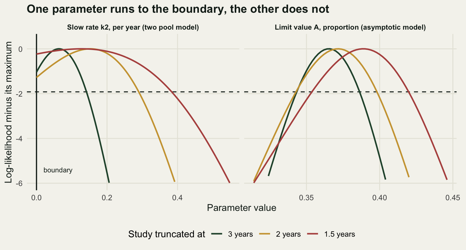
Early harvests buy the fast rate, late ones buy the slow rate
The profile is one study. The general statement behind it is that each rate is identified by the part of the curve where it is the thing that is happening, and that part is a stretch of calendar time the design either covers or does not. Measuring it needs replicates rather than one dataset, so here are two hundred simulated studies from the same process, once with the full seven harvests and then with harvests removed from each end in turn.
sim_one <- function(times, a = a_true, k1 = k1_true, k2 = k2_true) {
  t <- rep(times, each = n_bag)
  y <- m_two(t, a, k1, k2) + rnorm(length(t), 0, sd_true)
  s <- start_values(t, y)
  f <- fit_two_pool(t, y, s)
  c(f$par["k1"], f$par["k2"])
}

n_rep <- 200
rmse <- function(x, truth) sqrt(mean((x - truth)^2))

ends <- rbind(
  `all seven harvests` = harvest %in% harvest,
  `first harvest dropped` = harvest >= 0.5,
  `first two dropped` = harvest >= 0.75,
  `last harvest dropped` = harvest <= 2,
  `last two dropped` = harvest <= 1.5)

end_tab <- t(apply(ends, 1, function(keep) {
  set.seed(20260726)
  m <- t(replicate(n_rep, sim_one(harvest[keep])))
  c(harvests = sum(keep), first = min(harvest[keep]), last = max(harvest[keep]),
    rmse_k1 = rmse(m[, 1], k1_true), rmse_k2 = rmse(m[, 2], k2_true),
    median_k1 = median(m[, 1]), median_k2 = median(m[, 2]),
    k2_exactly_zero = sum(m[, 2] < 1e-6))
}))
print(round(end_tab, 4))
harvests first last rmse_k1 rmse_k2 median_k1 median_k2
all seven harvests 7 0.25 3.0 0.3903 0.0296 3.4846 0.0776
first harvest dropped 6 0.50 3.0 0.6654 0.0335 3.4926 0.0764
first two dropped 5 0.75 3.0 16.8316 0.0368 3.5285 0.0809
last harvest dropped 6 0.25 2.0 0.4706 0.0532 3.4880 0.0724
last two dropped 5 0.25 1.5 0.7020 0.0895 3.5222 0.0861
k2_exactly_zero
all seven harvests 2
first harvest dropped 5
first two dropped 8
last harvest dropped 23
last two dropped 51round(c(replicates = n_rep,
k1_cost_of_dropping_two_early =
end_tab["first two dropped", "rmse_k1"] /
end_tab["all seven harvests", "rmse_k1"],
k2_cost_of_dropping_two_early =
end_tab["first two dropped", "rmse_k2"] /
end_tab["all seven harvests", "rmse_k2"],
k1_cost_of_dropping_two_late =
end_tab["last two dropped", "rmse_k1"] /
end_tab["all seven harvests", "rmse_k1"],
k2_cost_of_dropping_two_late =
end_tab["last two dropped", "rmse_k2"] /
end_tab["all seven harvests", "rmse_k2"]), 4) replicates k1_cost_of_dropping_two_early
200.0000 43.1272
k2_cost_of_dropping_two_early k1_cost_of_dropping_two_late
1.2436 1.7987
k2_cost_of_dropping_two_late
3.0210 Dropping the three-month and six-month harvests multiplies the error in the fast rate by 43.13 and the error in the slow rate by only 1.24. By nine months the fast pool is nearly gone, and a design that starts there is asking the model to estimate a rate from the residue of a process it never observed. The median estimate is not the problem: it stays at 3.5285 against a truth of 3.5. The problem is that individual studies run away, and a root mean squared error of 16.83 per year is what a handful of runaway fits looks like when they are averaged with the well behaved ones.
Dropping the two-year and three-year harvests does the mirror image: the slow rate error is multiplied by 3.02 while the fast rate error is multiplied by 1.80.
The count in the last column is worth its own sentence. On the full design, 2 of the two hundred fits returned a slow rate of exactly zero: the optimiser walked to the boundary and stayed there, which is the two-pool model reporting that the litter has a permanent limit value. Cut the study to eighteen months and that count is 51. Nothing about the litter changed.
The number the two models disagree about
The generating process has no limit value. Everything in the bag decomposes, given a century. The asymptotic model fitted to the study reports a limit value of 0.3653. That number is not a small error in a parameter; it is a positive answer to a question whose true answer is zero, and the study has no way to say so.
A_hat <- unname(coef(fit_A)["A"])
cross <- log((1 - a_true) / A_hat) / k2_true
round(c(reported_limit_value = A_hat,
        true_limit_value = 0,
        mean_mass_at_the_last_harvest = as.numeric(mbar["3"]),
        true_mass_when_the_study_ended = m_two(3, a_true, k1_true, k2_true),
        year_the_true_curve_passes_the_reported_limit = cross,
        true_mass_remaining_at_20_years = m_two(20, a_true, k1_true, k2_true),
        percent_of_the_reported_limit_left_at_20_years =
          100 * m_two(20, a_true, k1_true, k2_true) / A_hat), 4)
reported_limit_value
0.3653
true_limit_value
0.0000
mean_mass_at_the_last_harvest
0.3546
true_mass_when_the_study_ended
0.3540
year_the_true_curve_passes_the_reported_limit
2.6072
true_mass_remaining_at_20_years
0.0909
percent_of_the_reported_limit_left_at_20_years
24.8722 The observed mean mass at the final harvest is 0.3546, which is already below the reported limit of 0.3653. The true curve passes that level in year 2.61, before the last bags came out of the ground. The study reported a floor that its own final harvest had gone through. By twenty years the true mass remaining is 0.0909, which is 24.87 per cent of the reported limit.
One dataset is one draw, so the next step is a sweep across the true slow rate, holding everything else fixed. Two hundred studies at each value, both models fitted to each, and two questions asked of the result: what limit value does the asymptotic model report, and how often does AIC prefer the two-pool model by more than two units.
k2_grid <- c(0.02, 0.05, 0.08, 0.15, 0.30)

sweep_one <- function(k2) {
  t <- rep(harvest, each = n_bag)
  y <- m_two(t, a_true, k1_true, k2) + rnorm(length(t), 0, sd_true)
  s <- start_values(t, y)
  f2p <- fit_two_pool(t, y, s)
  fas <- fit_asymptote(t, y, s)
  c(A = unname(fas$par["A"]), k2 = unname(f2p$par["k2"]),
    d = aic_by_hand(fas$rss, length(y), 2) - aic_by_hand(f2p$rss, length(y), 3))
}

sw <- t(sapply(k2_grid, function(k2) {
  set.seed(20260726)
  m <- t(replicate(n_rep, sweep_one(k2)))
  c(k2_true = k2, half_life = log(2) / k2,
    A_median = median(m[, "A"]), A_q10 = quantile(m[, "A"], 0.1),
    A_q90 = quantile(m[, "A"], 0.9),
    k2_median = median(m[, "k2"]),
    delta_aic_median = median(m[, "d"]),
    power = mean(m[, "d"] > 2))
}))
colnames(sw) <- c("k2_true", "half_life", "A_median", "A_q10", "A_q90",
                  "k2_median", "delta_aic_median", "power")
print(round(sw, 4))
k2_true half_life A_median A_q10 A_q90 k2_median delta_aic_median power
[1,] 0.02 34.6574 0.4315 0.4231 0.4428 0.0192 -1.4139 0.100
[2,] 0.05 13.8629 0.4053 0.3970 0.4166 0.0482 1.0606 0.395
[3,] 0.08 8.6643 0.3803 0.3712 0.3916 0.0776 4.2297 0.715
[4,] 0.15 4.6210 0.3253 0.3144 0.3381 0.1483 11.3037 0.955
[5,] 0.30 2.3105 0.2294 0.2167 0.2435 0.2967 17.7385 0.990At a true slow rate of 0.02 per year, a half-life of 34.66 years, the asymptotic model reports a median limit value of 0.4315 and AIC prefers the two-pool model in 10.00 per cent of the studies. At 0.08 per year, which is the process behind everything above, the reported limit is 0.3803 and the model comparison notices the second pool 71.50 per cent of the time. Only by 0.15 per year, a slow-pool half-life of 4.62 years, does the comparison become reliable at 95.50 per cent. The median reported limit at that point is still 0.3253, against a true limit of zero, because AIC noticing the second pool does not stop the other model from reporting its parameter.
That is the whole problem in one row of a table. The slow rates that matter, the ones that decide whether litter carbon is gone in decades or held for centuries, are exactly the rates a three-year study cannot distinguish from zero; and when it fails to distinguish them it does not return a wide interval on a limit value, it returns a tight interval on a limit value that does not exist. A reported limit value can be an artefact of a slow second pool plus a study that ended, and the model comparison on that study does not have the power to tell you which it is.
sw_df <- as.data.frame(sw)
pan <- c("Reported limit value A", "Share of studies where AIC picks two pools")
band <- data.frame(x = sw_df$k2_true, lo = sw_df$A_q10, hi = sw_df$A_q90,
                   panel = factor(pan[1], levels = pan))
both <- rbind(
  data.frame(x = sw_df$k2_true, y = sw_df$A_median,
             panel = factor(pan[1], levels = pan)),
  data.frame(x = sw_df$k2_true, y = sw_df$power,
             panel = factor(pan[2], levels = pan)))
zero_line <- data.frame(panel = factor(pan[1], levels = pan), y = 0)
half_line <- data.frame(panel = factor(pan[2], levels = pan), y = 0.5)

both$hue <- ifelse(both$panel == pan[1], te_pal$clay, te_pal$forest)

ggplot(both, aes(x, y)) +
  geom_ribbon(data = band, aes(x = x, ymin = lo, ymax = hi),
              inherit.aes = FALSE, fill = te_pal$sage, alpha = 0.45) +
  geom_hline(data = zero_line, aes(yintercept = y), colour = te_pal$ink,
             linewidth = 1) +
  geom_hline(data = half_line, aes(yintercept = y), colour = te_pal$ink,
             linetype = 2, linewidth = 0.6) +
  geom_line(colour = both$hue, linewidth = 1) +
  geom_point(colour = both$hue, size = 2.4) +
  geom_text(data = data.frame(panel = factor(pan[1], levels = pan),
                              x = 0.0205, y = 0.055,
                              lab = "true limit value"),
            aes(x = x, y = y, label = lab), inherit.aes = FALSE, hjust = 0,
            size = 3.1, colour = te_pal$ink) +
  facet_wrap(~panel, scales = "free_y") +
  scale_x_continuous(transform = "log10", breaks = k2_grid,
                     labels = sprintf("%.2f", k2_grid),
                     expand = expansion(mult = 0.09)) +
  labs(x = "True slow-pool rate k2 (per year)", y = NULL,
       title = "A limit value is reported whether or not there is one") +
  theme_te() +
  theme(strip.text = element_text(colour = te_pal$ink, face = "bold", size = 9),
        axis.text.x = element_text(size = 8.5),
        panel.spacing.x = unit(1.4, "lines"),
        plot.margin = margin(6, 14, 6, 6))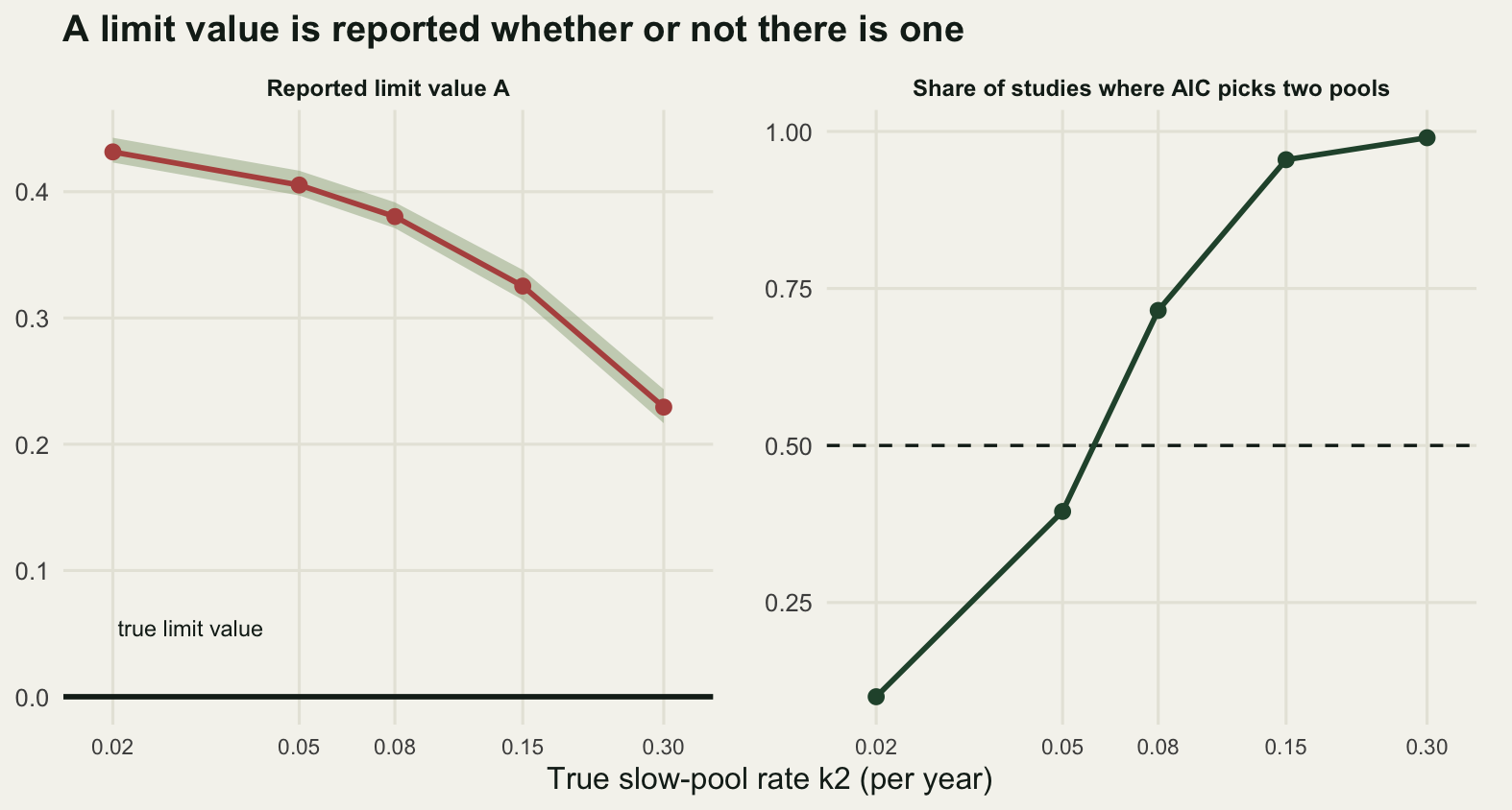
The reverse case is the one that decides whether this is a symmetric problem. Generate a study from a process that really does have a limit value, 0.45 of the mass held permanently, and fit the two-pool model to it. Does it invent a slow rate?
set.seed(20260726)
t_rev <- rep(harvest, each = n_bag)
y_rev <- m_asym(t_rev, 1 - a_true, k1_true) + rnorm(length(t_rev), 0, sd_true)
s_rev <- start_values(t_rev, y_rev)
f_rev_two <- fit_two_pool(t_rev, y_rev, s_rev)
f_rev_asym <- fit_asymptote(t_rev, y_rev, s_rev)

set.seed(20260726)
rev_many <- t(replicate(n_rep, {
  y <- m_asym(t_rev, 1 - a_true, k1_true) + rnorm(length(t_rev), 0, sd_true)
  f <- fit_two_pool(t_rev, y, start_values(t_rev, y))
  c(k2 = unname(f$par["k2"]))
}))

round(c(true_limit_value = 1 - a_true,
        asymptotic_fit_A = f_rev_asym$par["A"],
        asymptotic_fit_k = f_rev_asym$par["k"],
        two_pool_fit_k2 = f_rev_two$par["k2"],
        two_pool_fit_a = f_rev_two$par["a"],
        delta_aic_two_pool_minus_asymptotic =
          aic_by_hand(f_rev_two$rss, n_obs, 3) -
          aic_by_hand(f_rev_asym$rss, n_obs, 2),
        share_of_fits_with_k2_exactly_zero = mean(rev_many < 1e-6),
        k2_invented_median = median(rev_many),
        k2_invented_90th = quantile(rev_many, 0.9),
        half_life_implied_by_the_90th_percentile =
          log(2) / quantile(rev_many, 0.9)), 4)
true_limit_value
0.4500
asymptotic_fit_A.A
0.4375
asymptotic_fit_k.k
3.0934
two_pool_fit_k2.k2
0.0000
two_pool_fit_a.a
0.5625
delta_aic_two_pool_minus_asymptotic
2.0000
share_of_fits_with_k2_exactly_zero
0.5050
k2_invented_median
0.0000
k2_invented_90th.90%
0.0267
half_life_implied_by_the_90th_percentile.90%
25.9549 On this draw the two-pool model does not invent anything: it returns a slow rate of 0.0000, sits on the boundary, and reproduces the asymptotic fit exactly, which is why its AIC is worse by 2.00 units, the pure cost of one unused parameter. Across the two hundred replicates it lands exactly on the boundary in 50.50 per cent of them, and in the rest it invents a small one. Counting the zeros in, the ninetieth percentile of the rate it returns is 0.0267 per year, a half-life of 25.95 years.
So the two errors are not the same size. The two-pool model can return the asymptotic model, because the asymptotic model is a point in its parameter space and the optimiser reaches it. The asymptotic model cannot return the two-pool model, because the two-pool model is not in its parameter space at all. Fitting the wider model and looking at what happens to \(k_2\) is therefore the safer of the two habits, and the profile is the part that carries the information: an estimate of \(k_2\) of 0.0637 with an interval that starts at the boundary and reaches to 0.1400, more than twice the estimate, is a report of ignorance, and a limit value of 0.3653 with an interval 0.0420 wide is a report of confidence, from the same twenty-eight bags.
Design beats effort, and the schedule is free
Everything so far treats the harvest schedule as given. It is the one thing in a litterbag study that costs nothing to change: eight harvests are eight harvests whether they fall every four and a half months or not. Here are four schedules, all with eight harvests, all with four bags per harvest, all ending at three years.
Even spacing is the default in the notebook. Log spacing puts them at equal ratios of elapsed time, so half of them fall in the first eight months. The other two come from a power rule, \(t_i = 3(i/8)^p\), with \(p = 2\) pulling harvests towards the start and \(p = 0.5\) pushing them towards the end. All four schedules use the same random draws, so the comparison between them is paired and the differences are not Monte Carlo noise about which schedule got the easier datasets.
by_power <- function(n, p) 3 * (seq_len(n) / n)^p
by_log <- function(n, t1 = 0.125) exp(seq(log(t1), log(3), length.out = n))

schedules <- list(Even = by_power(8, 1), `Log spaced` = by_log(8),
                  `Front loaded` = by_power(8, 2),
                  `Back loaded` = by_power(8, 0.5))
print(round(do.call(rbind, schedules), 3))
[,1] [,2] [,3] [,4] [,5] [,6] [,7] [,8]
Even 0.375 0.750 1.125 1.500 1.875 2.250 2.625 3
Log spaced 0.125 0.197 0.310 0.488 0.768 1.210 1.905 3
Front loaded 0.047 0.188 0.422 0.750 1.172 1.688 2.297 3
Back loaded 1.061 1.500 1.837 2.121 2.372 2.598 2.806 3m10_true <- m_two(10, a_true, k1_true, k2_true)
sim_design <- function(times) {
t <- rep(times, each = n_bag)
y <- m_two(t, a_true, k1_true, k2_true) + rnorm(length(t), 0, sd_true)
f <- fit_two_pool(t, y, start_values(t, y))
c(f$par["k1"], f$par["k2"],
m10 = unname(m_two(10, f$par["a"], f$par["k1"], f$par["k2"])))
}
n_rep_d <- 300
design_rmse <- function(times) {
set.seed(20260726)
m <- t(replicate(n_rep_d, sim_design(times)))
c(k1 = rmse(m[, 1], k1_true), k2 = rmse(m[, 2], k2_true),
mass_at_10_years = rmse(m[, 3], m10_true))
}
sched_tab <- t(sapply(schedules, design_rmse))
print(round(sched_tab, 4)) k1 k2 mass_at_10_years
Even 0.4390 0.0278 0.0473
Log spaced 0.2892 0.0298 0.0523
Front loaded 0.3245 0.0284 0.0487
Back loaded 16.2333 0.0378 0.0688ratio_tab <- sweep(sched_tab, 2, sched_tab["Log spaced", ], "/")
print(round(ratio_tab, 3)) k1 k2 mass_at_10_years
Even 1.518 0.933 0.903
Log spaced 1.000 1.000 1.000
Front loaded 1.122 0.954 0.930
Back loaded 56.123 1.269 1.314round(c(replicates = n_rep_d, bags_in_every_design = 8 * n_bag,
true_mass_at_10_years = m10_true,
monte_carlo_error_on_each_rmse_percent = 100 / sqrt(2 * n_rep_d),
first_back_loaded_harvest_years = schedules[["Back loaded"]][1],
percent_of_the_fast_pool_gone_by_then =
100 * (1 - exp(-k1_true * schedules[["Back loaded"]][1]))), 4) replicates bags_in_every_design
300.0000 32.0000
true_mass_at_10_years monte_carlo_error_on_each_rmse_percent
0.2022 4.0825
first_back_loaded_harvest_years percent_of_the_fast_pool_gone_by_then
1.0607 97.5579 No schedule wins everything, which is not what I expected when I set this up. Taking log spacing as the reference, the even schedule’s error in the fast rate is 1.518 times log spacing’s, and its error in the slow rate is 0.933 times and its ten-year extrapolation 0.903 times. Log spacing buys the fast rate and sells the slow one. The front-loaded schedule is the compromise: 1.122 times log spacing on the fast rate, better than it on both of the others, and it is the only one of the three usable schedules that is never worst. Back loading loses on all three, and its fast rate error of 16.23 per year is not a number, it is a report that the parameter was not estimated: with the first bags coming up at 1.061 years the fast pool is 97.56 per cent gone before anything is weighed.
The Monte Carlo error on each of these root mean squared errors is about 4.08 per cent of its own value, so the differences of thirty and fifty per cent are real and the differences of five per cent are not worth reading.
lab_par <- c(k1 = "Fast rate k1", k2 = "Slow rate k2",
             mass_at_10_years = "Mass left at 10 years")
rat_df <- data.frame(
  schedule = factor(rep(rownames(ratio_tab), 3), levels = rownames(ratio_tab)),
  quantity = factor(rep(lab_par[colnames(ratio_tab)], each = nrow(ratio_tab)),
                    levels = unname(lab_par)),
  ratio = as.numeric(ratio_tab))
cap_at <- 1.72
rat_df$xnum <- as.numeric(rat_df$schedule) +
  (as.numeric(rat_df$quantity) - 2) * 0.2
off <- rat_df[rat_df$ratio > cap_at, ]
off$lab <- sprintf("off the scale at %.1f", off$ratio)
inn <- rat_df[rat_df$ratio <= cap_at, ]

ggplot(inn, aes(xnum, ratio, colour = quantity, shape = quantity)) +
  geom_hline(yintercept = 1, linetype = 2, colour = te_pal$ink,
             linewidth = 0.6) +
  geom_point(size = 3.4) +
  # the clipped point is a fast rate value, so it keeps the fast rate's glyph:
  # a hollow version of the circle, not the slow rate's triangle. The label
  # clears the marker rather than sitting on top of it.
  geom_point(data = off, aes(xnum, cap_at), inherit.aes = FALSE,
             shape = 1, size = 3.8, stroke = 1.2, colour = te_pal$clay) +
  geom_text(data = off, aes(xnum + 0.06, cap_at, label = lab),
            inherit.aes = FALSE, hjust = 1, vjust = -1.7, size = 3.1,
            colour = te_pal$ink) +
  scale_colour_manual(values = c(te_pal$clay, te_pal$forest, te_pal$gold),
                      name = NULL) +
  scale_shape_manual(values = c(16, 17, 15), name = NULL) +
  scale_x_continuous(breaks = seq_along(levels(rat_df$schedule)),
                     labels = levels(rat_df$schedule),
                     limits = c(0.5, 4.5)) +
  scale_y_continuous(transform = "log10", breaks = c(0.9, 1, 1.1, 1.25, 1.5),
                     labels = c("0.90", "1.00", "1.10", "1.25", "1.50"),
                     limits = c(0.87, 1.95)) +
  labs(x = NULL, y = "Error relative to the log-spaced schedule",
       title = "The schedule trades the fast rate against the slow one") +
  theme_te() +
  theme(plot.margin = margin(6, 14, 6, 6))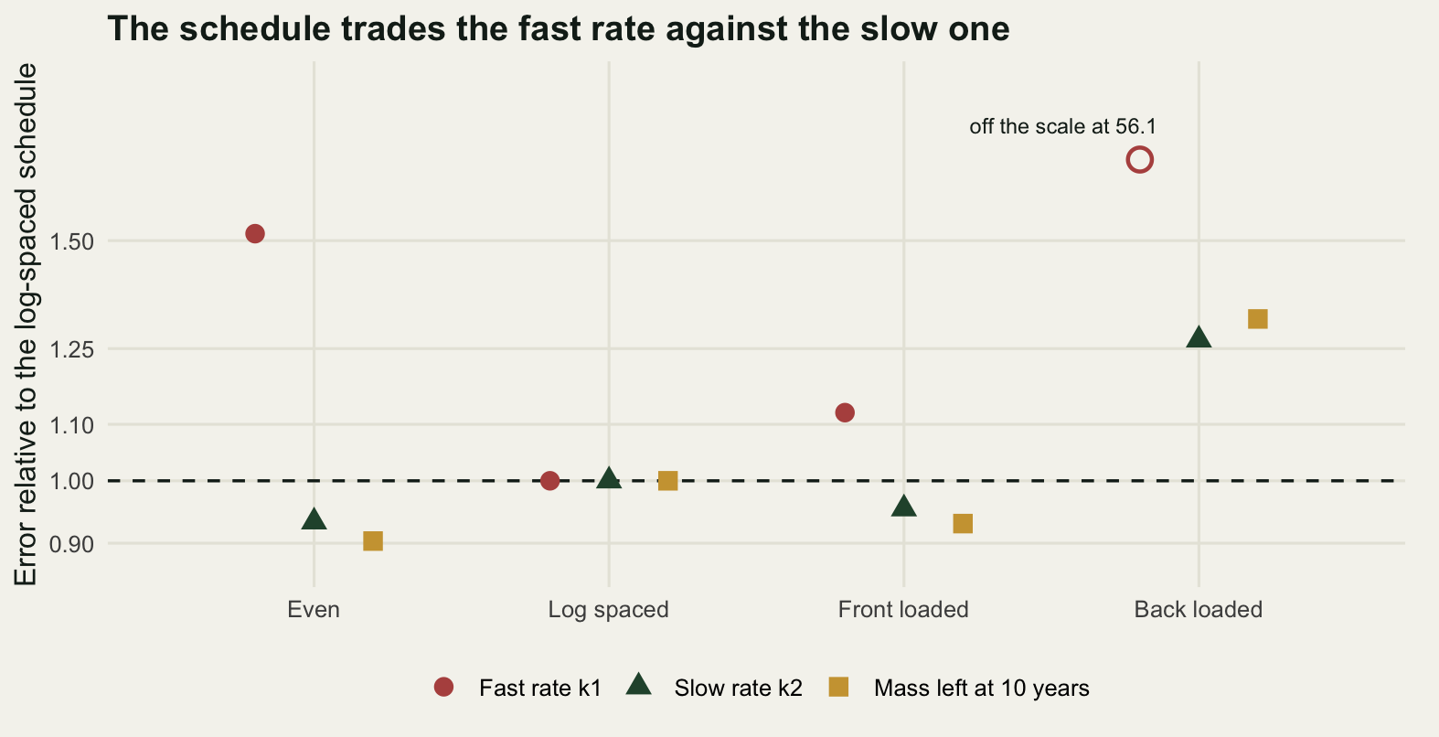
Now the question that makes this actionable. The schedule is free and harvests are not, so how many extra harvests would the even schedule need to reach the fast-rate error that log spacing gets for nothing? Run the even schedule at eight, ten, twelve, fourteen, sixteen, twenty and twenty-four harvests, fit the error against the harvest count on the log scale, and solve.
n_grid <- c(8, 10, 12, 14, 16, 20, 24)
even_curve <- t(sapply(n_grid, function(n) design_rmse(by_power(n, 1))))
rownames(even_curve) <- n_grid
print(round(even_curve, 4))
k1 k2 mass_at_10_years
8 0.4390 0.0278 0.0473
10 0.3758 0.0244 0.0408
12 0.3243 0.0231 0.0384
14 0.3292 0.0211 0.0350
16 0.2848 0.0212 0.0343
20 0.2419 0.0170 0.0291
24 0.2213 0.0165 0.0279b <- coef(lm(log(even_curve[, "k1"]) ~ log(n_grid)))
target <- sched_tab["Log spaced", "k1"]
n_needed <- exp((log(target) - b[1]) / b[2])
round(c(slope_of_error_against_harvests = b[2],
even_schedule_error_at_8 = even_curve["8", "k1"],
log_schedule_error_at_8 = target,
harvests_the_even_schedule_needs = n_needed,
extra_harvests = n_needed - 8,
extra_bags = (n_needed - 8) * n_bag,
percent_more_bags = 100 * (n_needed - 8) / 8), 4) slope_of_error_against_harvests.log(n_grid)
-0.6188
even_schedule_error_at_8
0.4390
log_schedule_error_at_8
0.2892
harvests_the_even_schedule_needs.(Intercept)
15.5248
extra_harvests.(Intercept)
7.5248
extra_bags.(Intercept)
30.0993
percent_more_bags.(Intercept)
94.0604 The error in the fast rate falls with the number of harvests at a rate of -0.619 on the log scale, a little steeper than the square root law, because extra harvests on an even schedule buy an earlier first harvest as well as more data. To reach the fast-rate error that log spacing gets from eight harvests, the even schedule needs 15.52 of them: 7.52 extra harvests, 30.10 extra litterbags, and 94.06 per cent more washing and weighing, for a result that a different line in the field notebook would have delivered on the original budget.
The honest version of that headline includes the trade. Adding harvests to the even schedule improves all three quantities at once; re-spacing eight harvests improves one and costs a little on the others. If the study exists to estimate the fast rate, or to compare litter types on early mass loss, re-space and pocket the saving. If it exists to extrapolate, the last harvest is what pays, and the money goes into keeping the site alive rather than into the first year.
The honest limit
Two things this analysis cannot do, and the second is the one that matters for the literature.
The first is mechanism. Nothing in a two-pool fit establishes that there are two chemically distinct pools. The model is a curve with three parameters, and other processes make the same curve. The standard alternative is a continuum of rates rather than two of them: litter is a mixture of compounds whose decay rates are drawn from a distribution, the fast ones go first, and the average rate of what is left falls through time without anything being partitioned. If the rates follow a gamma distribution with shape 0.55 and rate parameter 0.50, the mass remaining has a closed form, \(M(t) = (1 + t/\beta)^{-\alpha}\), which makes it cheap to check the simulator against the algebra before using it.
alpha <- 0.55
beta <- 0.5
m_gamma <- function(t) (1 + t / beta)^(-alpha)

set.seed(20260726)
k_draws <- rgamma(2e5, shape = alpha, rate = beta)
t_chk <- c(0.25, 1, 3, 10)
sim_mix <- sapply(t_chk, function(x) mean(exp(-k_draws * x)))
print(round(rbind(years = t_chk,
                  closed_form = m_gamma(t_chk),
                  average_of_200000_exponentials = sim_mix), 5))
[,1] [,2] [,3] [,4]
years 0.25000 1.00000 3.00000 10.00000
closed_form 0.80011 0.54649 0.34292 0.18740
average_of_200000_exponentials 0.79925 0.54536 0.34200 0.18647round(c(largest_difference = max(abs(m_gamma(t_chk) - sim_mix)),
largest_difference_as_percent =
100 * max(abs(m_gamma(t_chk) / sim_mix - 1)),
measurement_sd = sd_true), 5) largest_difference largest_difference_as_percent
0.00113 0.49868
measurement_sd
0.03000 set.seed(20260726)
y_cont <- m_gamma(tt) + rnorm(n_obs, 0, sd_true)
s_cont <- start_values(tt, y_cont)
f_cont_two <- fit_two_pool(tt, y_cont, s_cont)
f_cont_asym <- fit_asymptote(tt, y_cont, s_cont)
f_cont_true <- optim(c(log(alpha), log(beta)),
function(z) sum((y_cont - (1 + tt / exp(z[2]))^(-exp(z[1])))^2),
control = list(reltol = 1e-12, maxit = 3000))
round(c(aic_gamma_continuum = aic_by_hand(f_cont_true$value, n_obs, 2),
aic_two_pool = aic_by_hand(f_cont_two$rss, n_obs, 3),
aic_asymptotic = aic_by_hand(f_cont_asym$rss, n_obs, 2),
two_pool_minus_true_model = aic_by_hand(f_cont_two$rss, n_obs, 3) -
aic_by_hand(f_cont_true$value, n_obs, 2),
asymptotic_minus_true_model = aic_by_hand(f_cont_asym$rss, n_obs, 2) -
aic_by_hand(f_cont_true$value, n_obs, 2),
reported_limit_value = f_cont_asym$par["A"],
truth_at_30_years = m_gamma(30),
two_pool_prediction_at_10_years =
m_two(10, f_cont_two$par["a"], f_cont_two$par["k1"], f_cont_two$par["k2"]),
truth_at_10_years = m_gamma(10)), 4) aic_gamma_continuum aic_two_pool
-104.3371 -103.4814
aic_asymptotic two_pool_minus_true_model
-105.0056 0.8557
asymptotic_minus_true_model reported_limit_value.A
-0.6685 0.3268
truth_at_30_years two_pool_prediction_at_10_years.a
0.1042 0.1830
truth_at_10_years
0.1874 The average of two hundred thousand exponentials with gamma-distributed rates agrees with the closed form to within 0.0011 of the initial mass at every horizon, which is 0.04 of the measurement error on one bag, so the continuum data are what they claim to be. Fitted to them, the two-pool model comes within 0.86 AIC units of the true model, and the asymptotic model beats the true model by 0.67 units while reporting a limit value of 0.3268 for a process whose mass remaining at thirty years is 0.1042 and still falling. A three-parameter curve fitted to twenty-eight points cannot see the difference between two pools and a continuum, and the model that fits best here is the one that is wrong in the most expensive direction.
One more number is worth printing. The two-pool fit to continuum data predicts 0.1830 of the mass remaining at ten years against a truth of 0.1874, over a horizon three times the study length. Whether a wrong mechanism still predicts well outside the window is something you can check, one dataset at a time; whether its parameters mean what their names say is a different question, and a different standard of evidence.
The second limit is about time. A limit value is a statement about a horizon nobody observed. The profile interval for the limit value in this study, 0.3440 to 0.3860, is computed from data covering three years and describes the behaviour of the litter for ever. It is an extrapolation interval, and the assumption doing the work is not in the data at all: it is the choice of a model in which the curve has a horizontal asymptote. Change that choice to a model in which it does not and the same twenty-eight numbers give an interval on the slow rate whose lower end is zero and whose upper end is 0.1400. Both intervals are correct given their model. Only one of them tells you that the study did not settle the question.
The practical form of that is a rule about reporting rather than about fitting. If a limit value is reported, it should carry the length of the study next to it, because the number means “the fraction still there when we stopped, projected forward under a model that cannot decline”. Berg and Ekbohm fitted limit values to long-running needle litter series, and Adair and colleagues fitted a three-pool model across a multi-site decomposition experiment; both rest on series far longer than three years, which is the right way round. The measurement here says the same thing in the negative: three years and twenty-eight bags do not contain the information, and no amount of model selection can put it there.
Where to go next
The mass-remaining curve is only half of a decomposition study; what the litter releases is the other half, and turning a decay constant into a mass or carbon flux is the subject of mass loss and the carbon budget. When the fit itself misbehaves, which the boundary counts above show is a regular event for the two-pool model, checking a decomposition analysis collects the residual and influence checks that belong with these fits, and checking a nonlinear model covers the same ground for nonlinear fits in general.
If the flat ridge in the likelihood is the part that interested you, it is a general property rather than a decomposition problem, and starting values and identifiability takes it apart with simpler models where the geometry is easier to see. The mechanics of nls, including the self-starting models that make the fits above shorter to write, are in nonlinear regression with nls. And the AIC comparison that failed to separate the two models here is worth reading against model selection with AIC, which measures what delta values of two and four are actually worth on data of this size.
References
Olson JS 1963 Ecology 44(2):322-331 (10.2307/1932179)
Wieder RK, Lang GE 1982 Ecology 63(6):1636-1642 (10.2307/1940104)
Berg B, Ekbohm G 1991 Canadian Journal of Botany 69(7):1449-1456 (10.1139/b91-187)
Adair EC, Parton WJ, Del Grosso SJ, Silver WL, Harmon ME, Hall SA, Burke IC, Hart SC 2008 Global Change Biology 14(11):2636-2660 (10.1111/j.1365-2486.2008.01674.x)
Manzoni S, Pineiro G, Jackson RB, Jobbagy EG, Kim JH, Porporato A 2012 Soil Biology and Biochemistry 50:66-76 (10.1016/j.soilbio.2012.02.029)
Bolker BM 2008 Ecological Models and Data in R, Princeton University Press (ISBN 978-0-691-12522-0)