library(ggplot2)

te_pal <- list(forest = "#275139", green = "#2f8f63", sage = "#93a87f",
               clay = "#b5534e", gold = "#cda23f", line = "#dad9ca",
               ink = "#16241d", paper = "#f5f4ee")

theme_te <- function() {
  theme_minimal(base_size = 12) +
    theme(panel.grid.minor = element_blank(),
          panel.grid.major = element_line(colour = "#e7e6dc"),
          plot.background = element_rect(fill = "#f5f4ee", colour = NA),
          panel.background = element_rect(fill = "#f5f4ee", colour = NA),
          plot.title = element_text(face = "bold", colour = te_pal$ink),
          axis.title = element_text(colour = "#2c3a31"),
          plot.margin = margin(10, 18, 8, 10))
}

f2 <- function(x) sprintf("%.2f", x)
f4 <- function(x) sprintf("%.4f", x)
pc <- function(x) sprintf("%.2f", 100 * x)
pc0 <- function(x) sprintf("%.0f", 100 * x)
Mass loss and the carbon budget
R
decomposition
carbon
ecology tutorial
ggplot2
Litterbag mass loss is not carbon loss: measure in R the carbon concentration drift, soil contamination and mesh corrections hidden inside a decay constant.
The bags come back out of the beech stand in October, five years after they went in. Someone spends a fortnight picking roots and soil out of them under a lamp, they are dried at sixty-five degrees and weighed, and the numbers go into a spreadsheet with one column per harvest. A single exponential is fitted through the forty bags, five from each of eight harvests, k comes out close to 0.33 per year, and the regression gives it a standard error that puts a confidence interval of about nine per cent either side of it. That interval is what goes in the paper.
Then the same k is used twice more, and neither use is in the paper’s methods. It is multiplied by the standing litter carbon stock to get an annual carbon flux from the forest floor. And somewhere downstream, in a synthesis or a model calibration, it is inverted: a steady-state stock is computed as input divided by k, and compared with a measured stock, and that comparison is read as a test of something.
Both of those steps look like arithmetic. They are not. Between the mass on the balance and the carbon in the budget there are three multiplicative corrections, and this post measures all three. The first is that litter carbon concentration is not constant, so mass remaining times the initial carbon concentration is not carbon remaining. The second is that the bags came back with soil in them, and soil is mass. The third is that some of the mass which left the bag left as fragments, which is not decomposition, it is transport.
The result the post is built around: two of the three corrections are each larger than the whole confidence interval the study reports on k, and the net of all three is close to twice its half-width. That interval is a statement about how well those forty bags pin down the slope of a line. It is not a statement about whether the line is measuring the right quantity.
The litter here is simulated, with a two-fraction composition and a known carbon concentration in each fraction, because a simulated cohort comes with a truth column: the exact carbon remaining at every date, which no real litterbag study has. Fitting the decay curve itself, and the question of which error model the fit should assume, is the job of fitting litter decomposition curves; this post takes the fit as given and asks what the fitted number means.
Mass is not carbon, and the concentration moves
Leaf litter is not one substance. A useful minimum is two fractions with different carbon concentrations and different rates: a soluble and cellulosic fraction that goes quickly, and a lignified fraction that goes slowly. The carbon concentration of the two is not the same. Lignin is around sixty per cent carbon by mass; sugars and cellulose are nearer forty. So the fraction that disappears first is the carbon-poor one, and the litter left behind is richer in carbon than the litter that went in.
The litter below is beech-like: a labile fraction that is most of the initial dry mass and a lignified remainder with a higher carbon concentration and a rate an order of magnitude slower. The initial carbon concentration is the number a study measures once on the fresh material and then uses on every harvest.
f_lab <- 0.62; c_lab <- 0.437; k_lab <- 1.10
f_rec <- 0.38; c_rec <- 0.524; k_rec <- 0.135
c0 <- f_lab * c_lab + f_rec * c_rec

mass_rem <- function(t) f_lab * exp(-k_lab * t) + f_rec * exp(-k_rec * t)
carb_rem <- function(t) c_lab * f_lab * exp(-k_lab * t) + c_rec * f_rec * exp(-k_rec * t)

yr <- c(1, 2, 3)
tab_c <- rbind(dry_mass_remaining = mass_rem(yr),
               carbon_remaining_true = carb_rem(yr),
               carbon_inferred_from_mass = c0 * mass_rem(yr),
               shortfall_per_cent = 100 * (c0 * mass_rem(yr) / carb_rem(yr) - 1),
               carbon_concentration_left = carb_rem(yr) / mass_rem(yr))
colnames(tab_c) <- paste0("year_", yr)
print(round(tab_c, 4))
year_1 year_2 year_3
dry_mass_remaining 0.5384 0.3588 0.2763
carbon_remaining_true 0.2642 0.1820 0.1428
carbon_inferred_from_mass 0.2531 0.1686 0.1299
shortfall_per_cent -4.1966 -7.3484 -9.0441
carbon_concentration_left 0.4907 0.5073 0.5168round(c(labile_fraction_of_mass = f_lab,
labile_per_cent_of_initial_mass = 100 * f_lab,
lignified_per_cent_of_initial_mass = 100 * f_rec,
labile_carbon_concentration = c_lab,
lignified_carbon_concentration = c_rec,
labile_rate_per_year = k_lab,
lignified_rate_per_year = k_rec,
initial_carbon_concentration = c0,
concentration_at_five_years = carb_rem(5) / mass_rem(5),
concentration_rise_per_cent =
100 * (carb_rem(5) / mass_rem(5) / c0 - 1)), 4) labile_fraction_of_mass labile_per_cent_of_initial_mass
0.6200 62.0000
lignified_per_cent_of_initial_mass labile_carbon_concentration
38.0000 0.4370
lignified_carbon_concentration labile_rate_per_year
0.5240 1.1000
lignified_rate_per_year initial_carbon_concentration
0.1350 0.4701
concentration_at_five_years concentration_rise_per_cent
0.5229 11.2359 The labile fraction is 62 per cent of the initial dry mass at a carbon concentration of 0.4370, the lignified remainder sits at 0.5240, and the mixture starts at 0.4701. At one year the litter is down to 0.5384 of its dry mass and its carbon concentration has climbed to 0.4907. Multiplying mass remaining by the initial concentration therefore understates the carbon still in the bag by 4.20 per cent. At two years the shortfall is 7.35 per cent and at three years 9.04 per cent. By five years the concentration has reached 0.5229, a rise of 11.24 per cent on the fresh material.
The direction matters more than the size, and it is not an accident of these particular numbers. In almost any litter the fast fraction is the carbon-poor one, so the residue is carbon-enriched, so mass remaining times the initial concentration underestimates carbon remaining, so carbon loss is overstated. A study that never measures carbon on the retrieved material and simply scales its mass curve reports a carbon flux that is too large, and the error grows with time since litterfall, which is to say it grows fastest in the part of the curve a long study was run to reach.
tg <- seq(0, 5, by = 0.02)
lev <- c("Dry mass remaining", "Carbon remaining (true)",
         "Carbon inferred from mass", "Shortfall of the inferred carbon")
pan <- c("Left per gram of initial litter (g)",
         "Shortfall of the inferred carbon (per cent)")
shortfall <- function(t) 100 * (1 - c0 * mass_rem(t) / carb_rem(t))

cur <- rbind(
  data.frame(t = tg, y = mass_rem(tg),      series = lev[1], panel = pan[1]),
  data.frame(t = tg, y = carb_rem(tg),      series = lev[2], panel = pan[1]),
  data.frame(t = tg, y = c0 * mass_rem(tg), series = lev[3], panel = pan[1]),
  data.frame(t = tg, y = shortfall(tg),     series = lev[4], panel = pan[2]))
cur$series <- factor(cur$series, levels = lev)
cur$panel  <- factor(cur$panel, levels = pan)

mark <- data.frame(t = 3, y = shortfall(3), panel = factor(pan[2], levels = pan),
                   lab = sprintf("%.2f per cent at 3 years", shortfall(3)))

ggplot(cur, aes(t, y, colour = series, linetype = series)) +
  geom_line(linewidth = 1.05) +
  geom_point(data = mark, aes(t, y), inherit.aes = FALSE, size = 2.6,
             colour = te_pal$ink) +
  geom_text(data = mark, aes(t, y, label = lab), inherit.aes = FALSE,
            hjust = 1.08, vjust = -0.7, size = 3.2, colour = te_pal$ink) +
  facet_wrap(~panel, scales = "free_y") +
  scale_colour_manual(values = c(te_pal$sage, te_pal$forest, te_pal$clay,
                                 te_pal$gold), name = NULL) +
  scale_linetype_manual(values = c(1, 1, 2, 1), name = NULL) +
  scale_x_continuous(limits = c(0, 5.05), breaks = 0:5) +
  guides(colour = guide_legend(nrow = 2)) +
  labs(x = "Years since the bags went out", y = NULL,
       title = "The gap the mass column cannot show you") +
  theme_te() +
  theme(legend.position = "bottom", legend.key.width = unit(2.2, "lines"),
        strip.text = element_text(colour = te_pal$ink, face = "bold",
                                  size = 8.8))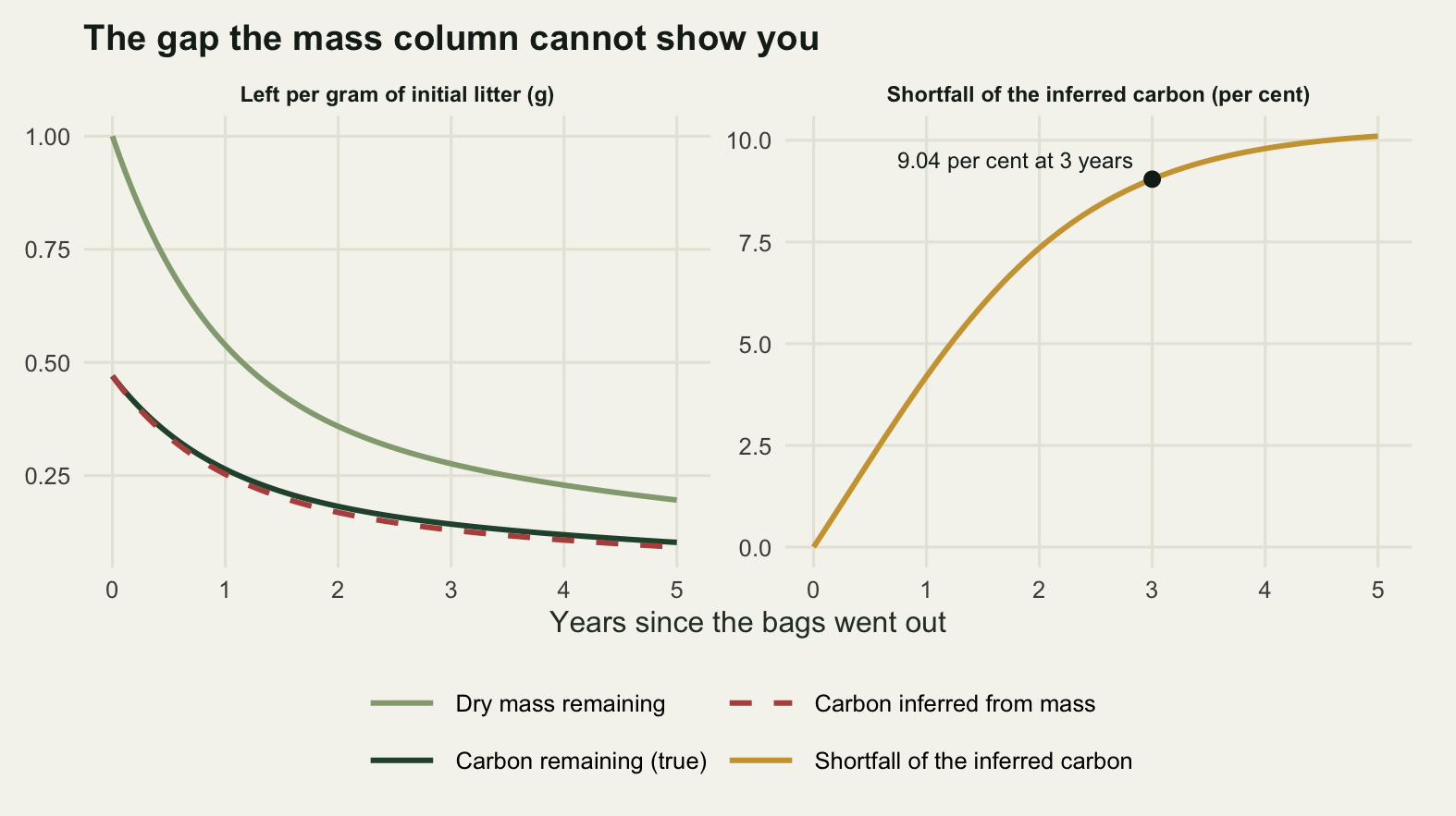
The same drift moves the decay constant. Fit Olson’s single exponential through the origin to the noise-free mass curve on the harvest schedule this post uses throughout, eight dates out to five years, then fit the identical model to the noise-free carbon curve. The two answers are not the same number.
harv <- c(0.25, 0.5, 1, 1.5, 2, 3, 4, 5)
n_rep <- 5

k_of  <- function(t, y) -coef(lm(log(y) ~ 0 + t))[[1]]
se_of <- function(t, y) summary(lm(log(y) ~ 0 + t))$coefficients[1, 2]

k_mass <- k_of(harv, mass_rem(harv))
k_carb <- k_of(harv, carb_rem(harv) / c0)

round(c(harvest_dates = length(harv),
        bags_per_date = n_rep,
        last_harvest_years = max(harv),
        k_fitted_to_dry_mass = k_mass,
        k_fitted_to_carbon = k_carb,
        carbon_correction_factor = k_carb / k_mass,
        per_cent_the_mass_fit_overstates = 100 * (k_mass / k_carb - 1)), 4)
harvest_dates bags_per_date
8.0000 5.0000
last_harvest_years k_fitted_to_dry_mass
5.0000 0.3831
k_fitted_to_carbon carbon_correction_factor
0.3565 0.9306
per_cent_the_mass_fit_overstates
7.4578 The mass fit gives 0.3831 per year and the carbon fit gives 0.3565 per year. Using the mass constant where the budget wants the carbon constant overstates the rate by 7.46 per cent. Hold that number: it is the smallest of the three corrections in this post, and it is the only one a laboratory can remove outright, by measuring carbon concentration on the retrieved material at every harvest instead of once at the start. That is a few hundred elemental analyser runs on material already dried and ground for weighing.
Ash, and why ash-free dry mass is not fussiness
A litterbag on a forest floor does not stay a discrete object. It settles, the leaves inside it flatten and mat, worm casts and mineral soil work in through the mesh and into the litter matrix itself, and by the last harvest what comes out of the bag is a composite of litter and soil that no amount of picking under a lamp fully separates. The correction is old and standard: burn a subsample at five hundred degrees, weigh the ash, and report ash-free dry mass. It is skipped often enough to be worth pricing.
The simulation below is deliberately simpler than the one above so that the answer is not in doubt. The litter is a single pool, so the true limit of the mass curve is zero by construction and there is no recalcitrant fraction anywhere in the generator. Mineral contamination accumulates as the bag flattens onto the soil surface, rising towards a plateau. Each bag is weighed with a twelve per cent lognormal error and the ash fraction is determined with an eight per cent error of its own.
k_single <- 0.35
a_max <- 0.08; a_rate <- 0.45
sd_bag <- 0.12; sd_ash <- 0.08

soil_on <- function(t) a_max * (1 - exp(-a_rate * t))

set.seed(20260726)
tb <- rep(harv, each = n_rep)
organic  <- exp(-k_single * tb)
raw_mass <- (organic + soil_on(tb)) * exp(rnorm(length(tb), 0, sd_bag))
ash_frac <- pmin((soil_on(tb) / (organic + soil_on(tb))) *
                   exp(rnorm(length(tb), 0, sd_ash)), 0.95)
afdm <- raw_mass * (1 - ash_frac)

k_raw_s  <- k_of(tb, raw_mass)
k_afdm_s <- k_of(tb, afdm)

round(c(true_k = k_single,
        contamination_plateau = a_max,
        bag_weighing_error = sd_bag,
        ash_determination_error = sd_ash,
        k_from_raw_dry_mass = k_raw_s,
        k_from_ash_free_dry_mass = k_afdm_s,
        raw_bias_per_cent = 100 * (k_raw_s / k_single - 1),
        ash_free_bias_per_cent = 100 * (k_afdm_s / k_single - 1),
        standard_error_raw = se_of(tb, raw_mass),
        standard_error_ash_free = se_of(tb, afdm),
        contamination_at_five_years = soil_on(5),
        organic_left_at_five_years = exp(-k_single * 5),
        ash_share_of_the_last_bags =
          soil_on(5) / (exp(-k_single * 5) + soil_on(5))), 4)
true_k contamination_plateau
0.3500 0.0800
bag_weighing_error ash_determination_error
0.1200 0.0800
k_from_raw_dry_mass k_from_ash_free_dry_mass
0.2956 0.3595
raw_bias_per_cent ash_free_bias_per_cent
-15.5393 2.7019
standard_error_raw standard_error_ash_free
0.0080 0.0078
contamination_at_five_years organic_left_at_five_years
0.0716 0.1738
ash_share_of_the_last_bags
0.2917 The litter decays at exactly 0.35 per year and the contamination rises towards 0.0800 of the initial litter mass. The raw-mass fit returns 0.2956, low by 15.54 per cent. The ash-free fit returns 0.3595, high by 2.70 per cent, which is sampling noise rather than bias. The mechanism is not subtle: contamination adds mass, added mass looks like mass that has not been lost, and the curve flattens. What makes it worth measuring rather than asserting is the size. At the last harvest only 0.1738 of the original litter is left as organic matter and 0.0716 of mineral soil has arrived, so 29.17 per cent of what goes on the balance at the final harvest is not litter at all.
The standard error on k is 0.0080 for the raw fit and 0.0078 for the ash-free one. The raw interval comfortably excludes the truth and the ash-free interval contains it, and nothing in the raw output announces which of the two situations you are in.
The spurious asymptote
The more damaging consequence is what contamination does to the shape of the curve rather than its slope. Contamination grows through the study and then levels off; the organic matter keeps declining. Their sum approaches the contamination plateau. So a mass curve with growing contamination does not head for zero, it heads for the amount of soil in the bag, and an asymptotic model fitted to it will find that plateau and report it as an undecomposable fraction of the litter.
asym_fit <- function(t, y) {
  ss <- function(p) {
    A <- plogis(p[1]); k <- exp(p[2])
    sum((y - ((1 - A) * exp(-k * t) + A))^2)
  }
  best <- NULL
  for (a0 in c(-4, -2, 0, 1)) for (k0 in log(c(0.08, 0.2, 0.5, 1))) {
    o <- optim(c(a0, k0), ss, control = list(reltol = 1e-12, maxit = 3000))
    if (is.null(best) || o$value < best$value) best <- o
  }
  c(limit_A = plogis(best$par[1]), k = exp(best$par[2]))
}

fit_clean_exact   <- asym_fit(harv, exp(-k_single * harv))
fit_dirty_exact   <- asym_fit(harv, exp(-k_single * harv) + soil_on(harv))
fit_raw_observed  <- asym_fit(tb, raw_mass)
fit_afdm_observed <- asym_fit(tb, afdm)

print(round(rbind(uncontaminated_exact = fit_clean_exact,
                  contaminated_exact = fit_dirty_exact,
                  raw_mass_observed = fit_raw_observed,
                  ash_free_observed = fit_afdm_observed), 4))
limit_A k
uncontaminated_exact 0.0000 0.3500
contaminated_exact 0.0772 0.3406
raw_mass_observed 0.0439 0.3225
ash_free_observed 0.0000 0.3531sweep_a <- sapply(c(0.00, 0.05, 0.08, 0.12, 0.16, 0.20), function(am) {
y <- exp(-k_single * harv) + am * (1 - exp(-a_rate * harv))
ft <- asym_fit(harv, y)
c(contamination_plateau = am, reported_limit = ft[["limit_A"]],
reported_k = ft[["k"]])
})
print(round(sweep_a, 4)) [,1] [,2] [,3] [,4] [,5] [,6]
contamination_plateau 0.00 0.0500 0.0800 0.1200 0.1600 0.2000
reported_limit 0.00 0.0483 0.0772 0.1155 0.1536 0.1914
reported_k 0.35 0.3444 0.3406 0.3353 0.3294 0.3228On uncontaminated noise-free data the asymptotic model recovers the truth exactly: a limit of 0.0000 and a rate of 0.3500. Add the contamination and nothing else, no measurement noise at all, and the same model reports a limit of 0.0772 of the initial litter mass, from a litter constructed with no undecomposable fraction whatever. On the noisy observed bags it reports 0.0439. Run the ash correction first and the reported limit falls to 0.0000, which is the boundary, which is right.
The sweep is the part to read twice. Across contamination plateaus from zero to 0.2000 of initial mass, the reported limit tracks the contamination almost one for one: at a plateau of 0.2000 the model reports 0.1914, and at 0.1200 it reports 0.1155. The asymptotic model is not detecting a recalcitrant pool. It is measuring the soil in the bag and giving it a biological name. Telling that apart from a real limit value is the subject of the recalcitrant pool and the asymptote, and the short version is that no amount of statistical care on the mass column can do it: the information that separates the two cases is in the muffle furnace, not in the model.
pts <- rbind(data.frame(t = tb, y = raw_mass, series = "Raw dry mass"),
             data.frame(t = tb, y = afdm, series = "Ash-free dry mass"))
pts$series <- factor(pts$series, levels = c("Raw dry mass", "Ash-free dry mass"))

A_hat <- fit_raw_observed[["limit_A"]]; k_hat <- fit_raw_observed[["k"]]
lin <- rbind(
  data.frame(t = tg, y = exp(-k_single * tg), series = "True curve (limit zero)"),
  data.frame(t = tg, y = exp(-k_afdm_s * tg), series = "Exponential on ash-free mass"),
  data.frame(t = tg, y = (1 - A_hat) * exp(-k_hat * tg) + A_hat,
             series = "Asymptotic model on raw mass"))
lin$series <- factor(lin$series, levels = c("True curve (limit zero)",
                                            "Exponential on ash-free mass",
                                            "Asymptotic model on raw mass"))
lin_hue <- c(te_pal$ink, te_pal$green, te_pal$gold)

ggplot() +
  geom_hline(yintercept = 0, colour = te_pal$ink, linewidth = 0.7) +
  geom_hline(yintercept = A_hat, linetype = 3, colour = te_pal$gold,
             linewidth = 1) +
  geom_point(data = pts, aes(t, y, colour = series), size = 1.9, alpha = 0.75) +
  geom_line(data = lin, aes(t, y, group = series, linetype = series),
            colour = lin_hue[as.integer(lin$series)], linewidth = 0.95) +
  annotate("text", x = 1.6, y = A_hat + 0.09, hjust = 0, size = 3.2,
           colour = te_pal$ink,
           label = sprintf("gold dotted line: limit reported from raw mass, %.4f",
                           A_hat)) +
  annotate("text", x = 0.05, y = -0.055, hjust = 0, size = 3.2,
           colour = te_pal$ink, label = "true limit of the litter curve: 0") +
  scale_colour_manual(values = c(te_pal$clay, te_pal$forest), name = NULL) +
  scale_linetype_manual(values = c(2, 1, 4), name = NULL) +
  scale_x_continuous(limits = c(0, 5.4), breaks = 0:5) +
  guides(colour = guide_legend(order = 1, ncol = 1),
         linetype = guide_legend(order = 2, ncol = 1,
                                 override.aes = list(colour = lin_hue,
                                                     linewidth = 0.95))) +
  coord_cartesian(ylim = c(-0.1, 1.25)) +
  labs(x = "Years since the bags went out",
       y = "Mass left per gram of initial litter",
       title = "Soil in the bag becomes a recalcitrant fraction in the model") +
  theme_te() +
  theme(legend.position = "bottom", legend.box = "horizontal",
        legend.key.width = unit(2.1, "lines"),
        legend.text = element_text(size = 8.4))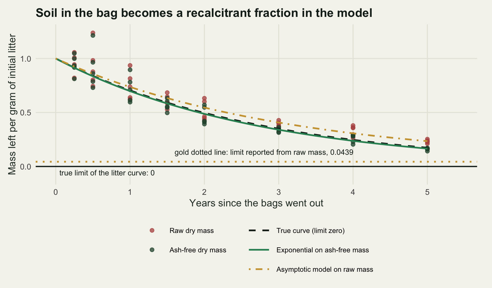
Fragmentation and the mesh
Mesh size is the choice that cannot be got right, because the mesh does two jobs and they want opposite answers. A fine mesh keeps the litter in: fragments that break off cannot leave, so the bag weighs what the cohort still is. It also keeps the soil fauna out, and a large share of litter mineralisation on a temperate forest floor is done by animals a half-millimetre mesh excludes. A coarse mesh lets the fauna in and lets the fragments out. Neither bag measures mineralisation.
Model the two directly. The fine bag mineralises at a reduced rate because the macrofauna are shut out, and loses a small amount as fine particles through the mesh. The coarse bag mineralises at the full field rate and loses a larger amount as fragments big enough to fall out. Both are fitted with the same single exponential on the same schedule, with the same weighing error as before.
k_min_true  <- 0.30
fauna_share <- 0.28
frag_fine   <- 0.02
frag_coarse <- 0.10

k_fine_true   <- k_min_true * (1 - fauna_share) + frag_fine
k_coarse_true <- k_min_true + frag_coarse
phi <- k_min_true / k_coarse_true

set.seed(20260726)
y_fine   <- exp(-k_fine_true * tb) * exp(rnorm(length(tb), 0, sd_bag))
y_coarse <- exp(-k_coarse_true * tb) * exp(rnorm(length(tb), 0, sd_bag))

k_fine   <- k_of(tb, y_fine)
k_coarse <- k_of(tb, y_coarse)

round(c(true_mineralisation_rate = k_min_true,
        fauna_share_of_mineralisation = fauna_share,
        fauna_per_cent_of_mineralisation = 100 * fauna_share,
        fragment_loss_fine_mesh = frag_fine,
        fragment_loss_coarse_mesh = frag_coarse,
        fine_mesh_estimate = k_fine,
        coarse_mesh_estimate = k_coarse,
        fine_mesh_error = k_fine - k_min_true,
        coarse_mesh_error = k_coarse - k_min_true,
        fine_mesh_error_per_cent = 100 * (k_fine / k_min_true - 1),
        coarse_mesh_error_per_cent = 100 * (k_coarse / k_min_true - 1),
        se_fine = se_of(tb, y_fine),
        se_coarse = se_of(tb, y_coarse),
        mineralised_share_of_coarse_mass_loss = phi,
        mineralised_per_cent_of_coarse_mass_loss = 100 * phi), 4)
true_mineralisation_rate
0.3000
fauna_share_of_mineralisation
0.2800
fauna_per_cent_of_mineralisation
28.0000
fragment_loss_fine_mesh
0.0200
fragment_loss_coarse_mesh
0.1000
fine_mesh_estimate
0.2421
coarse_mesh_estimate
0.3848
fine_mesh_error
-0.0579
coarse_mesh_error
0.0848
fine_mesh_error_per_cent
-19.2901
coarse_mesh_error_per_cent
28.2519
se_fine
0.0078
se_coarse
0.0061
mineralised_share_of_coarse_mass_loss
0.7500
mineralised_per_cent_of_coarse_mass_loss
75.0000 The true mineralisation rate constant, with the full decomposer community and no bag at all, is 0.30 per year, of which the macrofauna do 28 per cent. The fine bag reports 0.2421 per year and the coarse bag 0.3848. One is low by 19.29 per cent and the other high by 28.25 per cent, and the two standard errors are 0.0078 and 0.0061, so neither interval reaches the truth. The fine bag is closer here. That is the sentence to be careful with, because it is a property of these two numbers and not of mesh sizes.
The fine bag’s error is bounded by how much of the mineralisation the excluded animals were doing. The coarse bag’s error is the fragmentation rate, which depends on how brittle the litter gets and how large the holes are, and has no relation to the first quantity at all. So which bag wins is settled by a comparison between two unrelated site properties, and the crossover is worth writing down.
cross <- function(fs) abs(k_min_true * fs - frag_fine)
fs_grid <- c(0.10, 0.20, 0.28, 0.40, 0.55)
tab_x <- rbind(fauna_share_of_mineralisation = fs_grid,
               fauna_per_cent_of_mineralisation = 100 * fs_grid,
               fine_mesh_error = -(k_min_true * fs_grid - frag_fine),
               coarse_wins_below_this_fragment_rate = cross(fs_grid))
colnames(tab_x) <- paste0("case_", seq_along(fs_grid))
print(round(tab_x, 4))
case_1 case_2 case_3 case_4 case_5
fauna_share_of_mineralisation 0.10 0.20 0.280 0.4 0.550
fauna_per_cent_of_mineralisation 10.00 20.00 28.000 40.0 55.000
fine_mesh_error -0.01 -0.04 -0.064 -0.1 -0.145
coarse_wins_below_this_fragment_rate 0.01 0.04 0.064 0.1 0.145round(c(fragment_rate_used_here = frag_coarse,
crossover_at_this_fauna_share = cross(fauna_share),
one_over_the_mineralised_share = 1 / phi), 4) fragment_rate_used_here crossover_at_this_fauna_share
0.1000 0.0640
one_over_the_mineralised_share
1.3333 At the fauna share used above, the coarse bag is the better of the two whenever the fragment loss rate is below 0.0640 per year. The value here is 0.1000, so the fine bag wins, by a margin that a smaller mesh or a less brittle litter would reverse. Move the fauna share to 55 per cent and the crossover moves to 0.1450, which is above the fragment rate, and the coarse bag becomes the better estimator without anything about the bags changing.
There is a second point in the coarse-mesh number and it is the one that reaches the carbon budget. Of the mass the coarse bag loses, only 75 per cent was mineralised. The rest left the bag as fragments. That carbon is on the forest floor, a few centimetres away, and it is still carbon. The mass-loss arithmetic counts it as decomposed because the arithmetic knows only what is in the bag. For a budget that is a straight overestimate of the flux by a factor of 1.3333, and no statistical treatment of the mass column can see it, because the mass column is correct: the mass really did leave the bag.
From k to a stock, and the sensitivity that surprises people
The other use of k is inverted. At steady state, litter input I equals litter loss kX, so the standing stock is X = I / k. That is the arithmetic behind a large number of published litter and soil carbon stocks, and behind a larger number of model calibrations comparing a modelled stock with an observed one.
Both inputs carry error. Take a litter carbon input and a decay constant, each with a coefficient of variation of fifteen per cent. That is several times the within-study regression standard error on k, which in the contaminated study above was 2.70 per cent, and it is the right order for the uncertainty a budget should carry: replicate plots, litterfall traps that missed a mast year, one site standing in for a forest type. Both quantities are positive and skewed, so both are drawn from gamma distributions matched to those means and coefficients of variation.
I_bar <- 3.20; cv_I <- 0.15
k_bar <- 0.35; cv_k <- 0.15
n_draw <- 20000

rg <- function(n, m, cv) rgamma(n, shape = 1 / cv^2, rate = 1 / (m * cv^2))

set.seed(20260726)
k_draw <- rg(n_draw, k_bar, cv_k)
I_draw <- rg(n_draw, I_bar, cv_I)

X_both <- I_draw / k_draw
X_k    <- I_bar  / k_draw
X_I    <- I_draw / k_bar
X_at_mean <- I_bar / k_bar

round(c(draws = n_draw,
        mean_input_Mg_C_per_ha = I_bar,
        mean_k_per_year = k_bar,
        coefficient_of_variation = cv_k,
        stock_at_the_mean_k = X_at_mean,
        mean_simulated_stock = mean(X_both),
        median_simulated_stock = median(X_both),
        cv_of_the_stock = sd(X_both) / mean(X_both),
        first_order_prediction = sqrt(cv_I^2 + cv_k^2),
        sd_from_k_alone = sd(X_k),
        sd_from_input_alone = sd(X_I),
        ratio_of_the_two_sds = sd(X_k) / sd(X_I),
        upper_2_5_per_cent_point_k_alone = quantile(X_k, 0.975),
        upper_2_5_per_cent_point_input_alone = quantile(X_I, 0.975),
        jensen_gap_per_cent = 100 * (mean(X_both) / X_at_mean - 1),
        exact_gamma_prediction_per_cent = 100 * (1 / (1 - cv_k^2) - 1)), 4)
draws
20000.0000
mean_input_Mg_C_per_ha
3.2000
mean_k_per_year
0.3500
coefficient_of_variation
0.1500
stock_at_the_mean_k
9.1429
mean_simulated_stock
9.3573
median_simulated_stock
9.1502
cv_of_the_stock
0.2176
first_order_prediction
0.2121
sd_from_k_alone
1.4357
sd_from_input_alone
1.3816
ratio_of_the_two_sds
1.0391
upper_2_5_per_cent_point_k_alone.97.5%
12.5534
upper_2_5_per_cent_point_input_alone.97.5%
12.0579
jensen_gap_per_cent
2.3452
exact_gamma_prediction_per_cent
2.3018 The stock has a coefficient of variation of 21.76 per cent against a first-order prediction of 21.21 per cent, which is the calibration: the simulator and the formula agree, so what follows is a property of the ratio and not of the code.
Now the part usually stated wrongly, including in the plan for this post. To first order the stock is exactly as sensitive to a relative error in k as to the same relative error in I: both elasticities are one and the two contributions enter the variance formula symmetrically. What breaks the symmetry is the second order. The reciprocal is convex, so the same relative spread on k produces a wider and more skewed spread on X than it does applied to I. Here the standard deviation of the stock is 1.4357 from k alone against 1.3816 from input alone, a ratio of 1.0391. The upper tail is where it shows: the upper two and a half per cent point is 12.5534 Mg C per hectare from k alone and 12.0579 from input alone.
That is a smaller asymmetry than the framing “the reciprocal is the point” suggests, and the honest statement is that at the uncertainties a real budget carries the two error sources are close to interchangeable in size. The asymmetry grows quickly with the coefficient of variation, though, and a sweep is cheaper than an argument.
cv_grid <- c(0.05, 0.10, 0.15, 0.20, 0.30)
sw <- sapply(cv_grid, function(cv) {
  set.seed(20260726)
  a <- rg(n_draw, k_bar, cv); b <- rg(n_draw, I_bar, cv)
  c(cv = cv, cv_per_cent = 100 * cv,
    sd_ratio_k_over_input = sd(I_bar / a) / sd(b / k_bar),
    jensen_gap_per_cent = 100 * (1 / (1 - cv^2) - 1))
})
print(round(sw, 4))
[,1] [,2] [,3] [,4] [,5]
cv 0.0500 0.1000 0.1500 0.2000 0.3000
cv_per_cent 5.0000 10.0000 15.0000 20.0000 30.0000
sd_ratio_k_over_input 1.0013 1.0154 1.0391 1.0744 1.1934
jensen_gap_per_cent 0.2506 1.0101 2.3018 4.1667 9.8901At a coefficient of variation of 5 per cent the two are indistinguishable, a ratio of 1.0013. At 30 per cent the ratio is 1.1934. The practical reading: below about a fifth relative error, spend the effort on whichever of the two can be measured better, and do not choose on the grounds that one enters as a reciprocal.
The Jensen gap is the second consequence and it is unambiguous. Because 1/k is convex, the mean stock exceeds the stock computed at the mean k: 9.3573 against 9.1429 Mg C per hectare, a gap of 2.35 per cent, matching the exact gamma result 2.30 per cent. A synthesis that averages k across sites and then divides input by the average is not computing the average stock, and the same convexity argument in its more familiar setting is worked through in Jensen’s inequality and thermal variability.
pnx <- c("All the simulated stocks",
         "Zoom on the two reference lines")
zlo <- min(X_at_mean, mean(X_both)) - 0.5
zhi <- max(X_at_mean, mean(X_both)) + 0.5
mk_bars <- function(lo, hi, nb, pan) {
  br <- seq(lo, hi, length.out = nb + 1)
  h <- hist(X_both[X_both >= lo & X_both <= hi], breaks = br, plot = FALSE)
  data.frame(mid = h$mids, count = h$counts, w = br[2] - br[1], panel = pan)
}
hd <- rbind(mk_bars(floor(min(X_both)), ceiling(max(X_both)), 70, pnx[1]),
            mk_bars(zlo, zhi, 32, pnx[2]))
hd$panel <- factor(hd$panel, levels = pnx)
vl <- data.frame(x = rep(c(X_at_mean, mean(X_both)), 2),
                 lty = rep(c(2, 1), 2),
                 col = rep(c(te_pal$ink, te_pal$clay), 2),
                 panel = factor(rep(pnx, each = 2), levels = pnx))
notes <- data.frame(
  x = c(Inf, Inf, -Inf), y = Inf,
  hj = c(1.04, 1.04, -0.07), vj = c(1.7, 3.2, 1.7),
  col = c(te_pal$ink, te_pal$clay, te_pal$clay),
  lab = c(sprintf("dashed, at the mean k: %.4f", X_at_mean),
          sprintf("solid, the mean stock: %.4f", mean(X_both)),
          sprintf("Jensen gap:\n%.2f per cent",
                  100 * (mean(X_both) / X_at_mean - 1))),
  panel = factor(pnx[c(1, 1, 2)], levels = pnx))

ggplot(hd, aes(mid, count)) +
  geom_col(width = hd$w, fill = te_pal$sage, colour = NA) +
  geom_vline(data = vl, aes(xintercept = x), colour = vl$col,
             linetype = vl$lty, linewidth = 0.9) +
  geom_text(data = notes, aes(x = x, y = y, label = lab, hjust = hj,
                              vjust = vj),
            colour = notes$col, size = 3.2, lineheight = 0.95,
            inherit.aes = FALSE) +
  facet_wrap(~panel, scales = "free") +
  scale_y_continuous(expand = expansion(mult = c(0, 0.22))) +
  labs(x = "Steady-state litter carbon stock (Mg C per hectare)",
       y = "Simulated studies",
       title = "Dividing by an uncertain rate constant makes a skewed stock") +
  theme_te() +
  theme(strip.text = element_text(colour = te_pal$ink, face = "bold",
                                  size = 8.8))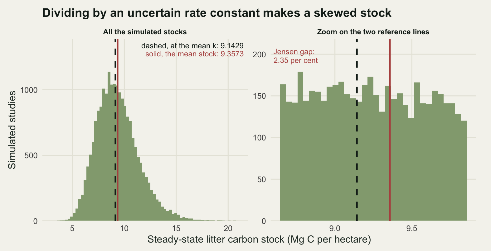
What steady state is worth
X = I / k assumes equilibrium. Litter input to most forests has not been constant for the last thirty years. Take an input rising at two per cent a year for thirty years, integrate the stock forward properly from an equilibrium start, and compare the true stock with what I / k reports using the input measured in the final year. Do it twice: once for a litter layer, once for a pool turning over seven times more slowly.
g_rate <- 0.02; n_yr <- 30

true_stock <- function(k, g, TT, I0)
  I0 * (exp(g * TT) - exp(-k * TT)) / (g + k) + (I0 / k) * exp(-k * TT)

ns <- sapply(c(litter_layer = 0.35, slow_pool = 0.05), function(kk) {
  Tr <- true_stock(kk, g_rate, n_yr, I_bar)
  Rp <- I_bar * exp(g_rate * n_yr) / kk
  c(k = kk, turnover_time_years = 1 / kk, true_stock = Tr,
    reported_by_I_over_k = Rp, overstated_per_cent = 100 * (Rp / Tr - 1))
})
print(round(ns, 4))
litter_layer slow_pool
k 0.3500 0.0500
turnover_time_years 2.8571 20.0000
true_stock 15.7589 87.3770
reported_by_I_over_k 16.6594 116.6156
overstated_per_cent 5.7142 33.4627round(c(input_growth_per_cent_per_year = 100 * g_rate,
years_of_growth = n_yr,
input_in_the_final_year = I_bar * exp(g_rate * n_yr)), 4)input_growth_per_cent_per_year years_of_growth
2.0000 30.0000
input_in_the_final_year
5.8308 For the litter layer the answer is smaller than the plan for this section expected. With k at 0.35 per year the pool turns over in 2.8571 years, so it tracks a slowly rising input almost completely, and I / k overstates the true stock by only 5.71 per cent, less than the Monte Carlo spread computed above. The steady-state assumption is not the problem for fast pools, and it gets blamed for discrepancies it cannot produce.
Take the same arithmetic to a slow pool and it changes character. At k of 0.05 per year the turnover time is twenty years, comparable with the period of change, the pool is still filling, and I / k overstates the true stock by 33.46 per cent. The rule that falls out is worth carrying: the steady-state error scales with how the turnover time compares with the timescale of the trend, so the same formula that is nearly harmless on the litter layer is badly wrong on the mineral soil carbon it is most often applied to.
Putting the three corrections together
Now the study from the top of the post, with all three problems at once. The litter is the two-fraction material from the first section, so the carbon concentration drifts. The bags are the coarse-mesh ones, so fragments leave. They came back with soil in them and were weighed without an ash correction. The standing litter carbon stock is measured separately and treated as known here, which flatters the estimate.
The three corrections multiply, and their product is exact rather than approximate: the ash correction takes the raw-mass constant to the true dry-mass constant, the fragment correction takes dry-mass loss to mineralised mass, and the carbon correction takes mineralised mass to mineralised carbon. Each was measured in its own section above. The chunk prints the product against the truth, but the residual only tests the ash step: the fragment factor and the fitted carbon constant cancel against the target, so what is left is the ash-corrected fit measured against the dry-mass constant.
X_C <- 3.60

set.seed(20260726)
org_study  <- mass_rem(tb)
raw_study  <- (org_study + soil_on(tb)) * exp(rnorm(length(tb), 0, sd_bag))
ashf_study <- pmin((soil_on(tb) / (org_study + soil_on(tb))) *
                     exp(rnorm(length(tb), 0, sd_ash)), 0.95)
afdm_study <- raw_study * (1 - ashf_study)

fit_study <- lm(log(raw_study) ~ 0 + tb)
k_raw  <- -coef(fit_study)[[1]]
se_raw <- summary(fit_study)$coefficients[1, 2]
ci_raw <- k_raw + c(-1, 1) * qt(0.975, length(tb) - 1) * se_raw
half_width <- (ci_raw[2] - k_raw) / k_raw

corr_ash  <- k_of(tb, afdm_study) / k_raw
corr_frag <- phi
corr_carb <- k_carb / k_mass
corr_all  <- corr_ash * corr_frag * corr_carb

k_target <- phi * k_carb

round(c(standing_litter_carbon_stock = X_C,
        k_from_raw_dry_mass = k_raw,
        standard_error = se_raw,
        ci_lower = ci_raw[1], ci_upper = ci_raw[2],
        ci_half_width_per_cent = 100 * half_width,
        ash_correction = corr_ash,
        fragment_correction = corr_frag,
        carbon_correction = corr_carb,
        product_of_the_three = corr_all,
        corrected_k = k_raw * corr_all,
        true_carbon_mineralisation_k = k_target,
        residual_after_all_three_per_cent =
          100 * (k_raw * corr_all / k_target - 1)), 4)
standing_litter_carbon_stock k_from_raw_dry_mass
3.6000 0.3265
standard_error ci_lower
0.0148 0.2967
ci_upper ci_half_width_per_cent
0.3564 9.1422
ash_correction fragment_correction
1.2018 0.7500
carbon_correction product_of_the_three
0.9306 0.8388
corrected_k true_carbon_mineralisation_k
0.2739 0.2674
residual_after_all_three_per_cent
2.4384 round(c(ash_correction_per_cent = 100 * (corr_ash - 1),
fragment_correction_per_cent = 100 * (corr_frag - 1),
carbon_correction_per_cent = 100 * (corr_carb - 1),
net_correction_per_cent = 100 * (corr_all - 1),
net_over_ci_half_width = abs(corr_all - 1) / half_width,
largest_single_over_ci_half_width =
max(abs(c(corr_ash, corr_frag, corr_carb) - 1)) / half_width,
flux_as_reported = k_raw * X_C,
flux_after_the_corrections = k_raw * corr_all * X_C,
true_flux = k_target * X_C,
overstatement_Mg_C_per_ha_per_year = (k_raw - k_target) * X_C,
overstatement_as_a_share_of_the_truth =
(k_raw - k_target) / k_target), 4) ash_correction_per_cent fragment_correction_per_cent
20.1804 -25.0000
carbon_correction_per_cent net_correction_per_cent
-6.9402 -16.1203
net_over_ci_half_width largest_single_over_ci_half_width
1.7633 2.7346
flux_as_reported flux_after_the_corrections
1.1756 0.9861
true_flux overstatement_Mg_C_per_ha_per_year
0.9626 0.2130
overstatement_as_a_share_of_the_truth
0.2213 The study reports k at 0.3265 per year with a confidence interval from 0.2967 to 0.3564, a half-width of 9.14 per cent. Set that beside the three corrections. The ash correction is 20.18 per cent upward, the fragment correction 25.00 per cent downward, the carbon correction 6.94 per cent downward. Two of the three are larger than the whole interval is wide, and the largest is 2.7346 times the half-width.
The net is 16.12 per cent downward, 1.7633 times the half-width. In flux terms the study reports 1.1756 Mg C per hectare per year from the forest floor when the truth is 0.9626, an overstatement of 0.2130 Mg C per hectare per year, or 22.13 per cent of the true flux. Applying all three corrections leaves a residual of 2.44 per cent against the truth, which is the sampling error in the ash-free fit and is the size an error ought to be.
steps <- c("Raw dry mass", "After ash", "After fragments", "After carbon")
ratio <- c(k_raw, k_raw * corr_ash, k_raw * corr_ash * corr_frag,
           k_raw * corr_all) / k_target
casc <- data.frame(step = factor(steps, levels = steps), ratio = ratio)
band_lab <- sprintf(
  "confidence interval on k: %.2f per cent either side, %.2f to %.2f",
  100 * half_width, 1 - half_width, 1 + half_width)

ggplot(casc, aes(step, ratio, group = 1)) +
  annotate("rect", xmin = -Inf, xmax = Inf,
           ymin = 1 - half_width, ymax = 1 + half_width,
           fill = te_pal$line, alpha = 0.8) +
  geom_hline(yintercept = c(1 - half_width, 1 + half_width),
             colour = te_pal$ink, linetype = 3, linewidth = 0.55) +
  geom_hline(yintercept = 1, colour = te_pal$ink, linewidth = 0.8) +
  geom_line(colour = te_pal$sage, linewidth = 1) +
  geom_point(size = 4, colour = te_pal$forest) +
  geom_text(aes(label = sprintf("%.2f", ratio)), vjust = -1.3, size = 3.6,
            colour = te_pal$ink) +
  annotate("text", x = 0.62, y = 1 - half_width - 0.055, hjust = 0, size = 3.4,
           colour = te_pal$ink, fontface = "bold", label = band_lab) +
  scale_x_discrete(expand = expansion(add = 0.45)) +
  scale_y_continuous(limits = c(0.80, 1.60), breaks = seq(0.8, 1.6, 0.1)) +
  labs(x = NULL, y = "Estimated flux divided by true flux",
       title = "Two of the three corrections beat the error bar") +
  theme_te()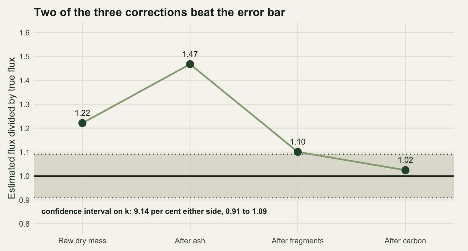
One more thing has to be said about that figure, because the near-cancellation in it is not a result. The ash correction pushes up and the other two push down, and how far they cancel depends entirely on how much soil got into the bags, which is a property of the site and the retrieval, not of the litter. Sweep it.
net_at <- sapply(c(0.00, 0.04, 0.08, 0.12, 0.16, 0.24), function(am) {
  s <- am * (1 - exp(-a_rate * tb))
  set.seed(20260726)
  r <- (org_study + s) * exp(rnorm(length(tb), 0, sd_bag))
  af <- pmin((s / (org_study + s)) * exp(rnorm(length(tb), 0, sd_ash)), 0.95)
  ca <- k_of(tb, r * (1 - af)) / k_of(tb, r)
  c(contamination_plateau = am, k_reported = k_of(tb, r), ash_correction = ca,
    net_correction_per_cent = 100 * (ca * corr_frag * corr_carb - 1))
})
print(round(net_at, 4))
[,1] [,2] [,3] [,4] [,5] [,6]
contamination_plateau 0.0000 0.0400 0.0800 0.1200 0.1600 0.2400
k_reported 0.3892 0.3559 0.3265 0.3002 0.2763 0.2342
ash_correction 1.0000 1.0980 1.2018 1.3128 1.4326 1.7054
net_correction_per_cent -30.2052 -23.3639 -16.1203 -8.3728 -0.0149 19.0257With clean bags the net correction is 30.21 per cent downward. At the contamination this study had it is 16.12 per cent downward. At a plateau of 0.1600 the three cancel to -0.0149 per cent, and at 0.2400 the net has changed sign and the study understates the flux by 19.03 per cent. The point of the cascade is not that the corrections are large in one direction. It is that a study applying none of them has a flux whose sign of error it cannot know, set by how muddy the bags were.
The honest limit
Everything above corrects arithmetic. A litterbag has a deeper problem that no arithmetic touches, and it is measurable, so here it is measured.
A litterbag holds a cohort. The forest floor holds a stock, and a stock at steady state is a mixture of cohorts of every age, weighted by how long each fraction persists. The slow fraction is over-represented in that mixture by the ratio of the residence times, so the standing litter is not compositionally the same material as fresh litterfall, and its turnover constant is not the one a fresh cohort gives.
stock_lab <- f_lab / k_lab
stock_rec <- f_rec / k_rec
k_eff_mass <- 1 / (stock_lab + stock_rec)
stock_carb <- c_lab * f_lab / k_lab + c_rec * f_rec / k_rec
k_eff_carb <- c0 / stock_carb

round(c(lignified_share_of_fresh_litter = f_rec,
        lignified_share_of_the_standing_stock =
          stock_rec / (stock_lab + stock_rec),
        cohort_k_dry_mass = k_mass,
        standing_stock_k_dry_mass = k_eff_mass,
        overstated_per_cent_mass = 100 * (k_mass / k_eff_mass - 1),
        cohort_k_carbon = k_carb,
        standing_stock_k_carbon = k_eff_carb,
        overstated_per_cent_carbon = 100 * (k_carb / k_eff_carb - 1),
        stock_per_unit_annual_input_years = stock_lab + stock_rec), 4)
lignified_share_of_fresh_litter lignified_share_of_the_standing_stock
0.3800 0.8332
cohort_k_dry_mass standing_stock_k_dry_mass
0.3831 0.2960
overstated_per_cent_mass cohort_k_carbon
29.4283 0.3565
standing_stock_k_carbon overstated_per_cent_carbon
0.2731 30.5479
stock_per_unit_annual_input_years
3.3785 The lignified fraction is 38 per cent of fresh litterfall and 83.32 per cent of the standing litter layer. The cohort fit over five years gives a carbon constant of 0.3565 per year; the constant that actually governs the standing stock is 0.2731 per year. Using the cohort number for the stock overstates the turnover by 30.55 per cent, larger than any single correction priced in the previous section. It is not in the cascade because it is not a correction to the litterbag. It is the statement that the litterbag was measuring a different object.
Three further limits have no number here, and saying so plainly is better than a hedge.
A bag changes the microclimate. Mesh holds moisture, the flattened mat inside a bag dries and wets on a different schedule from loose litter, and the direction depends on the site: wetter in a dry forest, less aerated in a wet one. That effect is a property of the stand, not of the arithmetic, and nothing here estimates it.
A bag excludes part of the decomposer community even at the coarsest mesh that will hold litter, and the fauna correction in the mesh section treated that exclusion as a known share of mineralisation. On a real site it is not known; it is the thing the mesh comparison was supposed to estimate, and the crossover measured above is why it cannot.
And the litter going into a bag has been collected, air dried, sometimes oven dried, and subsampled. Drying changes the leaching behaviour of the soluble fraction, which is a large part of the first year’s mass loss. The first harvest is the one most affected by that preparation and it is also the one that pulls hardest on a fitted k.
None of that is an argument against litterbags. It is an argument for reporting k as what it is: a mass-loss constant for a prepared cohort in a mesh bag, on a stated schedule, with a stated mesh and a stated ash treatment. The corrections priced here can only be applied by a reader who is told which of them the study already made.
Where to go next
The fit itself, and how much of the reported precision on k is an artefact of the assumed error model, is worked through in fitting litter decomposition curves. The limit value that turned up spuriously here is taken seriously in the recalcitrant pool and the asymptote, which separates the cases where a limit is real from the cases where it is contamination or a short study. Alongside both, checking a decomposition analysis is the diagnostic pass that catches most of what this post priced, and it is the cheapest of the three to run.
Two of the ideas here belong to wider families. The stock computation turns a rate into a density, and the general treatment of that step, including why the divisor belongs in the model rather than in a pre-computed response, is offsets for rates and densities. The interval on the corrected flux should be produced by resampling the whole chain rather than propagating the regression standard error alone, which is bootstrap confidence intervals. And if the carbon concentration is measured on the retrieved material rather than assumed, that measurement has an error of its own, which attenuates the correction it is meant to make: measurement error and regression dilution is the general form of that problem.
References
Olson JS 1963 Ecology 44(2):322-331 (10.2307/1932179)
Bocock KL, Gilbert OJW 1957 Plant and Soil 9(2):179-185 (10.1007/BF01398924)
Wieder RK, Lang GE 1982 Ecology 63(6):1636-1642 (10.2307/1940104)
Bradford MA, Tordoff GM, Eggers T, Jones TH, Newington JE 2002 Oikos 99(2):317-323 (10.1034/j.1600-0706.2002.990212.x)
Prescott CE 2010 Biogeochemistry 101(1-3):133-149 (10.1007/s10533-010-9439-0)
Adair EC, Parton WJ, Del Grosso SJ, Silver WL, Harmon ME, Hall SA, Burke IC, Hart SC 2008 Global Change Biology 14(11):2636-2660 (10.1111/j.1365-2486.2008.01674.x)
Robertson GP, Coleman DC, Bledsoe CS, Sollins P 1999 Standard Soil Methods for Long-Term Ecological Research, Oxford University Press (ISBN 978-0-19-512083-7)