---
title: "Soil carbon stocks and equivalent soil mass"
description: "Comparing soil carbon to a fixed sampling depth invents a difference whenever bulk density differs between treatments. The equivalent soil mass fix, in R."
date: "2026-08-06 14:00"
categories: [R, soil carbon, monitoring, carbon accounting, ecology tutorial]
image: thumbnail.png
image-alt: "Carbon concentration falling with cumulative soil mass, with two vertical lines marking where a fixed thirty centimetre core stops in a light soil and in a denser one."
---
A soil carbon stock is a concentration multiplied by a mass of soil. Everyone remembers the concentration. The mass is where the trouble is, because the standard protocol fixes the wrong thing: it fixes the depth. Sample both treatments to 30 cm, multiply concentration by bulk density by depth, and the treatment with the denser soil has been given more soil to hold carbon in.
That would be a curiosity if bulk density were a nuisance constant. It is not. Tillage, grazing, traffic, restoration planting and organic matter addition all change bulk density, so the treatments that shift carbon are exactly the treatments that shift the denominator. The difference this produces is not small compared with the effects people publish.
This post builds two soils that hold identical carbon per unit of soil mass, differing only in how tightly that soil is packed, and measures what a fixed depth comparison reports. Then it applies the equivalent soil mass correction and measures what is left. Nothing here is random: the whole thing is accounting, and the numbers are exact.
## Two soils with the same carbon
The generating model has to be set up carefully, and this is the part that decides whether the post is measuring anything. Carbon concentration is written as a function of **cumulative soil mass**, not of depth. That is what makes the two treatments genuinely identical: dig down through the same mass of soil in either one and you have passed through the same carbon. If concentration were written as a function of depth instead, the treatments would really differ in carbon and there would be nothing to detect.
```{r setup}
#| message: false
#| warning: false
library(ggplot2)

te_paper  <- "#f5f4ee"
te_ink    <- "#16241d"
te_body   <- "#2c3a31"
te_forest <- "#275139"
te_rust   <- "#b5534e"
te_gold   <- "#c9b458"
te_line   <- "#dad9ca"

theme_datasheet <- function() {
  theme_minimal(base_size = 12) +
    theme(plot.background  = element_rect(fill = te_paper, colour = NA),
          panel.background = element_rect(fill = te_paper, colour = NA),
          panel.grid.major = element_line(colour = te_line, linewidth = 0.3),
          panel.grid.minor = element_blank(),
          text             = element_text(colour = te_body),
          plot.title       = element_text(colour = te_ink, face = "bold"),
          axis.text        = element_text(colour = te_body))
}

# concentration in g C per kg soil, as a function of cumulative soil mass (Mg/ha)
conc  <- function(m, pr) pr[["b"]] + pr[["a"]] * exp(-pr[["k"]] * m)
# carbon stock in Mg C per ha down to cumulative mass M
stock <- function(M, pr) (pr[["a"]] * (1 - exp(-pr[["k"]] * M)) / pr[["k"]] +
                          pr[["b"]] * M) / 1000
# cumulative soil mass in Mg per ha at a given depth in cm
mass_to <- function(bd, d_cm) bd * (d_cm / 100) * 10000

bd_light <- 1.30            # g per cubic cm, the reference treatment
bd_dense <- 1.456           # twelve per cent denser
depth    <- 30              # cm, the sampled depth in both

m_light <- mass_to(bd_light, depth)
m_dense <- mass_to(bd_dense, depth)
c(mass_light = m_light, mass_dense = m_dense, extra = m_dense - m_light)
```
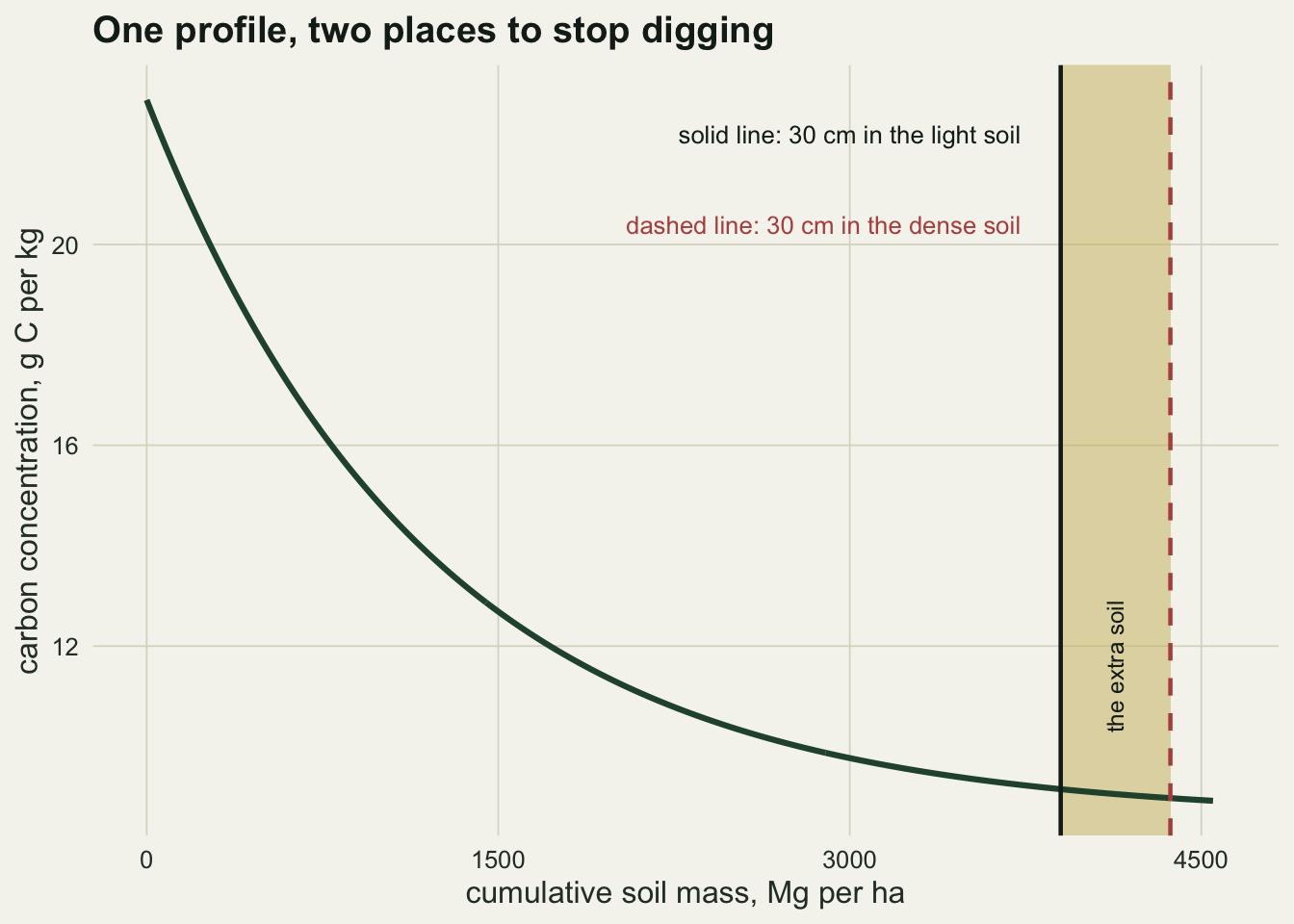
Sampling to 30 cm collects `r sprintf("%.0f", m_light)` Mg of soil per hectare in the light treatment and `r sprintf("%.0f", m_dense)` in the dense one. The core is the same length; the dense treatment simply gives up `r sprintf("%.0f", m_dense - m_light)` Mg more soil per hectare, and that soil arrives with carbon in it.
The profile itself is a surface enrichment decaying towards a mineral background. One number fixes the shape, the ratio of surface concentration to the concentration at the bottom of the reference core, and the whole profile is then scaled so that the reference mass holds exactly 50 Mg C per hectare.
```{r profile}
make_profile <- function(ratio, k, target = 50, M = m_light) {
  e <- exp(-k * M)
  if (ratio == 1) {
    a1 <- 0; b1 <- 1
  } else {
    a1 <- 1; b1 <- (1 - ratio * e) / (ratio - 1)
  }
  pr <- list(a = a1, b = b1, k = k)
  f  <- target / stock(M, pr)
  list(a = a1 * f, b = b1 * f, k = k)
}

pr <- make_profile(ratio = 2.5, k = 1 / 1200)
round(c(surface = conc(0, pr), at_reference_mass = conc(m_light, pr),
        stock_light = stock(m_light, pr), stock_dense = stock(m_dense, pr)), 3)
```
The surface holds `r sprintf("%.1f", conc(0, pr))` g C per kg and the bottom of the core `r sprintf("%.1f", conc(m_light, pr))`, which is an ordinary arable profile. Both treatments carry that identical curve. Yet the fixed depth stocks are `r sprintf("%.2f", stock(m_light, pr))` and `r sprintf("%.2f", stock(m_dense, pr))` Mg C per hectare, a difference of `r sprintf("%.2f", stock(m_dense, pr) - stock(m_light, pr))` Mg per hectare that belongs entirely to the extra slab of soil.
```{r fig-profile}
#| fig-cap: "Carbon concentration against cumulative soil mass. Both treatments follow the same curve, so they hold the same carbon per unit of soil. The vertical lines mark where a thirty centimetre core stops in each, and the shaded band is the extra soil the denser treatment contributes."
#| fig-alt: "A falling curve of carbon concentration against cumulative soil mass, from about twenty three grams per kilogram at the surface to about nine at the base of the core. A solid vertical line marks the light treatment at three thousand nine hundred megagrams per hectare and a dashed line the dense treatment at four thousand three hundred and sixty eight, with the strip between them shaded."
gm <- data.frame(m = seq(0, 4550, length.out = 400))
gm$conc <- conc(gm$m, pr)

ggplot(gm, aes(m, conc)) +
  annotate("rect", xmin = m_light, xmax = m_dense, ymin = -Inf, ymax = Inf,
           fill = te_gold, alpha = 0.45) +
  geom_line(linewidth = 1.1, colour = te_forest) +
  geom_vline(xintercept = m_light, linewidth = 0.8, colour = te_ink) +
  geom_vline(xintercept = m_dense, linewidth = 0.8, colour = te_rust,
             linetype = "dashed") +
  annotate("text", x = m_light - 170, y = 22.2, hjust = 1, size = 3.4,
           colour = te_ink, label = "solid line: 30 cm in the light soil") +
  annotate("text", x = m_light - 170, y = 20.4, hjust = 1, size = 3.4,
           colour = te_rust, label = "dashed line: 30 cm in the dense soil") +
  annotate("text", x = (m_light + m_dense) / 2, y = 11.6, hjust = 0.5,
           size = 3.2, colour = te_ink, angle = 90,
           label = "the extra soil") +
  scale_x_continuous(breaks = seq(0, 4500, 1500), limits = c(0, 4600)) +
  labs(x = "cumulative soil mass, Mg per ha",
       y = "carbon concentration, g C per kg",
       title = "One profile, two places to stop digging") +
  theme_datasheet()
```
## Where the phantom comes from, and how big it gets
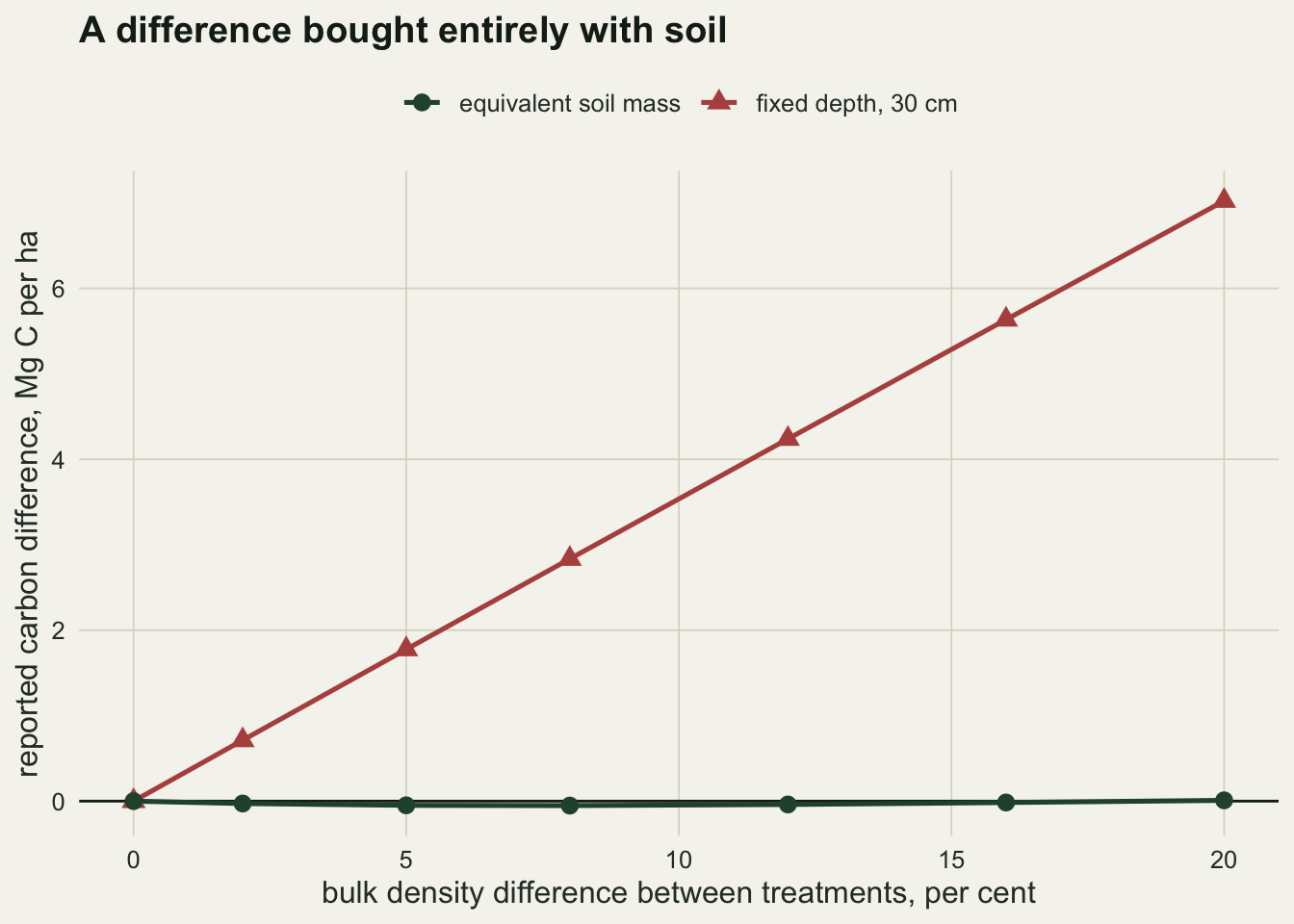
For a profile with no vertical gradient at all the arithmetic collapses to something worth stating plainly: the reported difference is the bulk density difference, exactly. Twelve per cent denser soil reports twelve per cent more carbon. A gradient softens that, because the extra soil comes from the bottom of the core where concentration is lowest, so the steeper the enrichment the smaller the phantom.
```{r shapes}
shapes <- list("uniform"   = c(ratio = 1.0,  k = 1 / 1500),
               "weak"      = c(ratio = 1.5,  k = 1 / 1500),
               "typical"   = c(ratio = 2.5,  k = 1 / 1200),
               "strong"    = c(ratio = 5.0,  k = 1 / 800),
               "very strong" = c(ratio = 12.0, k = 1 / 450))

shape_tab <- do.call(rbind, lapply(names(shapes), function(nm) {
  s  <- shapes[[nm]]
  p2 <- make_profile(s[["ratio"]], s[["k"]])
  sl <- stock(m_light, p2); sd_ <- stock(m_dense, p2)
  data.frame(shape = nm, surface = conc(0, p2), base = conc(m_light, p2),
             phantom = sd_ - sl, per_cent = 100 * (sd_ - sl) / sl)
}))
print(data.frame(shape_tab[1], round(shape_tab[-1], 3)), row.names = FALSE)
```
Every row holds `r sprintf("%.0f", stock(m_light, pr))` Mg C per hectare in the reference mass, so the only thing changing down the table is how that carbon is arranged. The phantom runs from `r sprintf("%.2f", min(shape_tab$phantom))` Mg per hectare under a strong surface enrichment up to `r sprintf("%.2f", max(shape_tab$phantom))` under none, which is `r sprintf("%.1f", min(shape_tab$per_cent))` to `r sprintf("%.1f", max(shape_tab$per_cent))` per cent of the stock. The uniform row is the identity: `r sprintf("%.3f", max(shape_tab$per_cent))` per cent reported against a bulk density difference of `r sprintf("%.3f", 100 * (bd_dense / bd_light - 1))` per cent.
Those are field trial numbers, not rounding. Published sequestration under a management change is commonly one to five Mg C per hectare accumulated over years of measurement.
## The correction, on the layer data you already have
The equivalent soil mass approach compares the treatments at the same cumulative soil mass rather than the same depth. You still sample by depth, because that is what an auger does, but you convert each layer to the soil mass it contained and accumulate. Cumulative carbon is then a function of cumulative mass in both treatments, and the comparison is read off at a common reference mass.
```{r layers}
layer_table <- function(bd, pr, bounds = c(0, 10, 20, 30)) {
  m <- mass_to(bd, bounds)
  data.frame(top = head(bounds, -1), bottom = bounds[-1],
             layer_mass = diff(m), mass_cum = m[-1],
             layer_c = diff(stock(m, pr)), c_cum = stock(m, pr)[-1])
}

lt_light <- layer_table(bd_light, pr)
lt_dense <- layer_table(bd_dense, pr)
print(round(lt_light, 2), row.names = FALSE)
print(round(lt_dense, 2), row.names = FALSE)
```
The two tables have the same depths and different masses in every layer. Cumulative carbon against cumulative mass is a smooth increasing function, so interpolating it at the reference mass is well behaved; a monotone spline keeps it from overshooting between the sampled points.
```{r esm}
esm_stock <- function(lt, m_ref) {
  f <- splinefun(c(0, lt$mass_cum), c(0, lt$c_cum), method = "monoH.FC")
  f(m_ref)
}

m_ref <- lt_light$mass_cum[nrow(lt_light)]     # the lighter treatment sets the reference
fixed <- lt_dense$c_cum[3] - lt_light$c_cum[3]
corr  <- esm_stock(lt_dense, m_ref) - esm_stock(lt_light, m_ref)

round(c(reference_mass = m_ref,
        equivalent_depth_cm = 100 * m_ref / (bd_dense * 10000),
        fixed_depth_difference = fixed,
        esm_difference = corr), 3)
```
At the reference mass of `r sprintf("%.0f", m_ref)` Mg per hectare the dense treatment has to be read at `r sprintf("%.1f", 100 * m_ref / (bd_dense * 10000))` cm rather than 30, and the reported difference falls from `r sprintf("%+.3f", fixed)` to `r sprintf("%+.3f", corr)` Mg per hectare. The residue is interpolation error between three sampled layers, and it is `r sprintf("%.0f", abs(fixed / corr))` times smaller than the artefact it replaced.
## What it does to a real effect
The comparison above had nothing to find. The case that matters is the one where something did happen and the density moved as well, which is the usual situation, because the practice that builds carbon also loosens the soil or the practice that compacts it also buries residue.
```{r real-effect}
pr_gain <- pr
pr_gain$b <- pr$b + 1000 * 2 / m_ref        # a genuine 2 Mg/ha, spread through the profile

lt_gain <- layer_table(bd_dense, pr_gain)
truth   <- stock(m_ref, pr_gain) - stock(m_ref, pr)

round(c(true_gain = truth,
        fixed_depth_reports = lt_gain$c_cum[3] - lt_light$c_cum[3],
        esm_reports = esm_stock(lt_gain, m_ref) - esm_stock(lt_light, m_ref)), 3)
```
A real gain of `r sprintf("%.1f", truth)` Mg C per hectare, in a treatment that is also `r sprintf("%.0f", 100 * (bd_dense / bd_light - 1))` per cent denser, is reported by the fixed depth calculation as `r sprintf("%.3f", lt_gain$c_cum[3] - lt_light$c_cum[3])`. The effect is real and the number is more than three times too large. Equivalent soil mass returns `r sprintf("%.3f", esm_stock(lt_gain, m_ref) - esm_stock(lt_light, m_ref))`.
This is the reason the correction is not a fussy detail about null results. A fixed depth stock is not a noisy version of the right answer; it is the right answer plus a term proportional to the density change, and that term does not shrink when the study gets bigger.
```{r sweep}
sweep_bd <- do.call(rbind, lapply(c(0, 2, 5, 8, 12, 16, 20), function(d) {
  bd2 <- bd_light * (1 + d / 100)
  l2  <- layer_table(bd2, pr)
  data.frame(bd_difference = d, bulk_density = bd2,
             fixed_depth = l2$c_cum[3] - lt_light$c_cum[3],
             esm = esm_stock(l2, m_ref) - esm_stock(lt_light, m_ref))
}))
round(sweep_bd, 3)
```
```{r fig-sweep}
#| fig-cap: "Reported carbon difference between two treatments holding identical carbon, against the bulk density difference between them. The fixed depth calculation rises with the density difference; the equivalent soil mass calculation stays on zero."
#| fig-alt: "Two lines against bulk density difference from zero to twenty per cent. The fixed depth line rises steadily from zero to about seven megagrams of carbon per hectare, while the equivalent soil mass line lies flat on the zero reference line across the whole range."
long <- rbind(
  data.frame(bd = sweep_bd$bd_difference, y = sweep_bd$fixed_depth,
             method = "fixed depth, 30 cm"),
  data.frame(bd = sweep_bd$bd_difference, y = sweep_bd$esm,
             method = "equivalent soil mass"))

ggplot(long, aes(bd, y, colour = method, shape = method)) +
  geom_hline(yintercept = 0, colour = te_ink, linewidth = 0.5) +
  geom_line(linewidth = 0.9) +
  geom_point(size = 2.9) +
  scale_colour_manual(values = c("fixed depth, 30 cm" = te_rust,
                                 "equivalent soil mass" = te_forest)) +
  scale_shape_manual(values = c(16, 17)) +
  labs(x = "bulk density difference between treatments, per cent",
       y = "reported carbon difference, Mg C per ha",
       colour = NULL, shape = NULL,
       title = "A difference bought entirely with soil") +
  theme_datasheet() +
  theme(legend.position = "top")
```
## Choosing the reference mass, which is a real decision
The reference mass has to be one that every treatment actually reached, and the safe choice is the lightest treatment's sampled mass. Take the heavier one instead and the light treatment has to be extended past the soil that was collected, which means extrapolating the cumulative curve rather than interpolating it.
```{r reference-choice}
m_ref_high <- lt_dense$mass_cum[nrow(lt_dense)]

round(c(reference_mass = m_ref_high,
        light_sampled_to = lt_light$mass_cum[3],
        extrapolated = esm_stock(lt_light, m_ref_high),
        truth = stock(m_ref_high, pr),
        reported_difference = esm_stock(lt_dense, m_ref_high) -
                              esm_stock(lt_light, m_ref_high)), 3)
```
Extrapolating the light treatment `r sprintf("%.0f", m_ref_high - lt_light$mass_cum[3])` Mg per hectare beyond its deepest sample overshoots the truth by `r sprintf("%.3f", esm_stock(lt_light, m_ref_high) - stock(m_ref_high, pr))` Mg per hectare, and the reported difference becomes `r sprintf("%+.3f", esm_stock(lt_dense, m_ref_high) - esm_stock(lt_light, m_ref_high))` where the truth is zero. That is far better than the fixed depth answer and far worse than the correct reference choice, and the sign has flipped, which is the part that would confuse a reader.
How finely the profile was cut also matters, because the interpolation is only as good as the points it runs through.
```{r layer-count}
by_layers <- do.call(rbind, lapply(c(2, 3, 4, 6), function(nl) {
  bounds <- seq(0, depth, length.out = nl + 1)
  ll <- layer_table(bd_light, pr, bounds)
  ld <- layer_table(bd_dense, pr, bounds)
  mr <- ll$mass_cum[nl]
  data.frame(layers = nl, layer_thickness_cm = depth / nl,
             esm_difference = esm_stock(ld, mr) - esm_stock(ll, mr))
}))
round(by_layers, 4)
```
Two thick layers leave `r sprintf("%.3f", abs(by_layers$esm_difference[1]))` Mg per hectare of interpolation error; six thin ones leave `r sprintf("%.3f", abs(by_layers$esm_difference[nrow(by_layers)]))`. Both are far smaller than the artefact they replace, so the correction is worth doing even on coarse data, but the layer scheme is the accuracy limit once the density problem is gone.
## What to record
Record the mass, not just the concentration. For every layer that means the depth interval, the oven dry mass of fine soil actually recovered from a known volume, and the coarse fragment content, because those three are what convert a concentration into a stock. A dataset that reports only carbon per cent by depth cannot be corrected afterwards by anyone, including the person who collected it.
Sample deeper than the depth you intend to compare. The reference mass has to sit inside the sampled range of every treatment, and the cheapest way to guarantee that is one extra layer below the zone of interest.
Report the bulk densities alongside the stocks. If they differ between treatments and the paper reports a fixed depth stock, the reader can work out the direction of the bias, and if they do not differ then the correction changes nothing and saying so costs one sentence.
## Honest limits
The correction needs soil that was sampled deeper than the reference mass, so it cannot be applied to an archive of fixed depth stocks where the deepest layer is the comparison depth. That is the main reason the older literature cannot simply be recomputed, and it is why the recommendation is about the next sampling campaign rather than the last one.
Coarse fragments are the second denominator, and they behave the same way. A stock calculated on whole soil rather than on the fine earth fraction carries the stone content of the plot inside it, and stone content varies over short distances in exactly the glacial and colluvial soils where field trials get sited.
The interpolation is a modelling choice. A monotone spline was used here and a cubic or a piecewise linear fit gives slightly different answers at the reference mass; with thin layers the choice hardly matters, and with two thick ones it becomes part of the uncertainty rather than a detail of the arithmetic.
Nothing above is stochastic. There is no sampling error in these numbers, which flatters the correction: in a real trial both the concentration and the density are estimated from a handful of cores, and the equivalent soil mass calculation propagates the density error into the reference mass as well as into the stock. The point of the exercise is that the fixed depth bias is not a variance problem, so more cores do not remove it, but a real study still has to carry the variance on top.
Finally, the model here holds carbon strictly as a function of soil mass. Real compaction does redistribute carbon vertically as well as compress the soil, and untangling a genuine redistribution from a packing change needs the profile, not a single stock number.
## References
Ellert BH, Bettany JR 1995 Canadian Journal of Soil Science 75(4):529-538 (10.4141/cjss95-075)
Wendt JW, Hauser S 2013 European Journal of Soil Science 64(1):58-65 (10.1111/ejss.12002)
von Haden AC, Yang WH, DeLucia EH 2020 Global Change Biology 26(7):3759-3770 (10.1111/gcb.15124)
Lee J, Hopmans JW, Rolston DE, Baer SG, Six J 2009 Agriculture Ecosystems and Environment 134(3-4):251-256 (10.1016/j.agee.2009.07.006)
## Related tutorials
- [Mass loss and the carbon budget](../mass-loss-and-the-carbon-budget/)
- [Closure and spurious correlation](../closure-and-spurious-correlation/)
- [Splicing a monitoring series](../splicing-a-monitoring-series/)
- [Offsets for rates and densities](../offsets-for-rates-and-densities/)