library(ggplot2)

te_pal <- list(forest = "#275139", green = "#2f8f63", sage = "#93a87f",
               clay = "#b5534e", gold = "#cda23f", line = "#dad9ca",
               ink = "#16241d", paper = "#f5f4ee")

theme_te <- function() {
  theme_minimal(base_size = 12) +
    theme(panel.grid.minor = element_blank(),
          panel.grid.major = element_line(colour = "#e7e6dc"),
          plot.background = element_rect(fill = "#f5f4ee", colour = NA),
          panel.background = element_rect(fill = "#f5f4ee", colour = NA),
          plot.title = element_text(face = "bold", colour = te_pal$ink),
          axis.title = element_text(colour = te_pal$ink),
          legend.position = "bottom")
}Checking a decomposition analysis
R
decomposition
model checking
ecology tutorial
ggplot2
Four checks on a litterbag decomposition analysis in R: bags nested in plots, comparing k between treatments, the fixed intercept, and extrapolated numbers.
The analysis arrives finished. Six harvests, a hundred and twenty mesh bags, mass remaining logged and regressed on time, and a decay constant of about eight tenths per year with a standard error in the third decimal place. The treatment contrast is significant. The report says the litter in the thinned plots decomposes twenty per cent faster than the litter in the controls, and it gives a time to ninety five per cent mass loss for the soil carbon section.
Every step of that is what the textbooks say to do, and four separate things in it are wrong. The standard error is too small by a factor that the design fixes and the fit never sees. The treatment comparison is done by a route whose stated error rate is not its actual error rate. The curve is forced through a point the litter did not start at. And the headline quantity, the time to ninety five per cent loss, sits outside the window the bags were ever in.
This post runs four checks on that analysis, one per section, each one a measurement that can come back clean. They are: whether the bags in a plot count as separate bags, whether the treatment comparison is the test it claims to be, whether the intercept can be fixed at one and detected if it should not have been, and how far the extrapolated number is from the data holding it up. Each check ends in a number, and each number is produced by code in the page.
The data are simulated, for the usual reason: a simulated litterbag study comes with a truth column, so an estimate can be scored instead of admired. The parameters are ordinary. A decay constant of eight tenths per year, a two-year study with six harvests, log-scale bag noise of about a fifth, and plots that differ from each other in decay rate by about fifteen per cent are all inside the range that turns up in published litterbag work.
Three neighbouring posts hold the machinery this one attacks. Fitting litter decomposition curves sets out Olson’s exponential, the two estimators and what the assumed error model costs. The recalcitrant pool and the asymptote covers what happens when one exponential is not enough. Mass loss and the carbon budget deals with the other half of the problem, which is whether the mass a litterbag loses is the carbon the ecosystem loses. Nothing here re-derives the fit. The fit is taken as given, and what is tested is everything between the fit and a sentence in a report.
The study under test
Ten plots. Six harvests at three, six and nine months and then at one, one and a half and two years. Two bags per plot per harvest, so one hundred and twenty bags in total, which is a study on the generous side of the litterbag literature.
The generator has three parts. Every plot gets its own decay constant, drawn around the true value with a standard deviation that stands for microclimate, litter quality and how the bags were pegged down. Every bag gets multiplicative noise on the log scale, which covers weighing, root picking and the fragments that fell out through the mesh. Mass remaining at time t in plot p is therefore exp(-k_p * t) times a lognormal error, and the fit throughout is the log-linear one through the origin, which is the estimator most litterbag papers use.
k_true <- 0.8
harvest <- c(0.25, 0.5, 0.75, 1, 1.5, 2)
tau_plot <- 0.12
sig_bag <- 0.18

fit_origin <- function(y, t) -sum(t * y) / sum(t^2)

round(c(true_k = k_true, harvests = length(harvest),
        plot_sd_of_k = tau_plot,
        plot_sd_as_percent_of_k = 100 * tau_plot / k_true,
        bag_sd_on_the_log_scale = sig_bag,
        mass_left_at_the_last_harvest = exp(-k_true * max(harvest)),
        mass_left_at_the_first_harvest = exp(-k_true * min(harvest))), 4)
true_k harvests
0.8000 6.0000
plot_sd_of_k plot_sd_as_percent_of_k
0.1200 15.0000
bag_sd_on_the_log_scale mass_left_at_the_last_harvest
0.1800 0.2019
mass_left_at_the_first_harvest
0.8187 The bags come back holding 0.8187 of their initial mass at the first harvest and 0.2019 at the last, so the study covers a bit under two thirds of the decay. The between-plot standard deviation of 0.12 is 15.0000 per cent of the decay constant itself, which is unremarkable: plots a hundred metres apart differ in litter moisture by more than that.
Check 1: the bags in a plot are not separate bags
Two bags lifted from the same plot on the same morning share the plot’s microclimate, the same person’s handling, the same drying oven and usually the same batch of starting material. The analysis pools all one hundred and twenty of them and fits one line. The design says the plot is the unit that was randomised; the fit says the bag is.
That mismatch is old ground in general, and this post does not re-argue it. Pseudoreplication in ecology sets out what the error is and nested counts, pseudoreplication and GLMMs fits the mixed model that handles it properly. What is measured here is the specific damage to a decay constant, and the specific fix, which does not need a mixed model at all.
The measurement is a straight comparison. Over replicates, the standard error the pooled fit prints is compared with the standard deviation the estimate actually has. The ratio between them is the square root of the design effect, and the total bag count divided by the design effect is the number of independent bags the study really bought. The whole thing is swept across allocations of the same one hundred and twenty bags: from two plots with ten bags per harvest to twenty plots with one.
set.seed(20260726)
n_rep <- 2000

sim_alloc <- function(P, nb, R) {
  tp <- rep(harvest, each = nb)
  st2 <- sum(tp^2)
  np <- length(tp)
  N <- P * np
  tv <- rep(tp, P)
  pid <- rep(seq_len(P), each = np)
  tc_n <- qt(0.975, N - 1)
  tc_p <- qt(0.975, P - 1)
  kn <- se_n <- cov_n <- kp_m <- cov_p <- gap <- numeric(R)
  for (i in seq_len(R)) {
    u <- rnorm(P, 0, tau_plot)
    y <- -(k_true + u[pid]) * tv + rnorm(N, 0, sig_bag)
    kh <- fit_origin(y, tv)
    res <- y + kh * tv
    se <- sqrt(sum(res^2) / (N - 1) / sum(tv^2))
    kps <- as.numeric(tapply(seq_len(N), pid,
                             function(j) fit_origin(y[j], tv[j])))
    m <- mean(kps)
    sp <- sd(kps) / sqrt(P)
    kn[i] <- kh
    se_n[i] <- se
    kp_m[i] <- m
    gap[i] <- abs(kh - m)
    cov_n[i] <- abs(kh - k_true) <= tc_n * se
    cov_p[i] <- abs(m - k_true) <= tc_p * sp
  }
  c(plots = P, bags_per_plot_per_harvest = nb, bags = N,
    reported_se = mean(se_n), actual_sd = sd(kn),
    ratio = sd(kn) / mean(se_n),
    effective_bags = N / (sd(kn) / mean(se_n))^2,
    coverage_pooled = mean(cov_n), coverage_plot_means = mean(cov_p),
    theory_actual_sd = sqrt(tau_plot^2 / P + sig_bag^2 / (P * st2)),
    theory_reported_se = sqrt(tau_plot^2 * (1 - 1 / P) / N + sig_bag^2 / (P * st2)),
    largest_gap_between_the_two_estimates = max(gap))
}

allocs <- list(c(2, 10), c(4, 5), c(5, 4), c(10, 2), c(20, 1))
nest <- t(sapply(allocs, function(a) sim_alloc(a[1], a[2], n_rep)))
rownames(nest) <- paste(sapply(allocs, `[`, 1), "plots")
main <- nest["10 plots", ]

print(c(replicates = n_rep))
replicates
2000 print(round(nest[, c("plots", "bags_per_plot_per_harvest", "reported_se",
"actual_sd", "ratio", "effective_bags")], 4)) plots bags_per_plot_per_harvest reported_se actual_sd ratio
2 plots 2 10 0.0159 0.0832 5.2352
4 plots 4 5 0.0169 0.0620 3.6744
5 plots 5 4 0.0170 0.0554 3.2688
10 plots 10 2 0.0175 0.0403 2.3091
20 plots 20 1 0.0177 0.0303 1.7154
effective_bags
2 plots 4.3785
4 plots 8.8880
5 plots 11.2308
10 plots 22.5064
20 plots 40.7791print(round(nest[, c("plots", "coverage_pooled", "coverage_plot_means",
"largest_gap_between_the_two_estimates")], 5)) plots coverage_pooled coverage_plot_means
2 plots 2 0.3020 0.9480
4 plots 4 0.4150 0.9465
5 plots 5 0.4535 0.9490
10 plots 10 0.6235 0.9405
20 plots 20 0.7505 0.9495
largest_gap_between_the_two_estimates
2 plots 0
4 plots 0
5 plots 0
10 plots 0
20 plots 0print(round(nest[, c("plots", "reported_se", "theory_reported_se",
"actual_sd", "theory_actual_sd")], 5)) plots reported_se theory_reported_se actual_sd theory_actual_sd
2 plots 2 0.01588 0.01611 0.08315 0.08602
4 plots 4 0.01686 0.01701 0.06195 0.06164
5 plots 5 0.01696 0.01719 0.05543 0.05549
10 plots 10 0.01745 0.01753 0.04030 0.04049
20 plots 20 0.01766 0.01770 0.03029 0.03032print(round(c(variance_ratio_four_plots_over_twenty_plots =
(nest["4 plots", "actual_sd"] / nest["20 plots", "actual_sd"])^2), 4))variance_ratio_four_plots_over_twenty_plots
4.1832 Read the ten-plot row, which is the design as described. The pooled fit reports a standard error of 0.0175. The estimate’s actual standard deviation over 2000 replicates is 0.0403. The ratio is 2.3091, so the interval printed by summary is a bit under half the width it should be, and the one hundred and twenty bags are worth 22.5064 independent bags.
The closed form agrees, which matters because it means the simulator and the algebra are describing the same study. The actual standard deviation should be the square root of the plot variance divided by the number of plots plus the bag term, giving 0.04049 against a simulated 0.04030, and the reported standard error should be 0.01753 against a simulated 0.01745.
The consequence is the coverage. A nominal ninety five per cent interval from the pooled fit contains the true k in 62.4 per cent of replicates.
The fix costs nothing. Fit k separately in each plot, then treat the ten plot-level estimates as the data: their mean is the estimate and their standard deviation over the square root of ten is the standard error. That interval covers in 94.0 per cent of replicates. No mixed model, no new package, ten numbers and a t.test.
There is a detail worth pausing on. The plot-mean estimate is not a different estimate. In a balanced design the mean of the per-plot slopes and the slope from pooling every bag are the same number: the largest gap between them anywhere in 2000 replicates of the ten-plot design is 0.00000. Nothing about the point estimate changes. What changes is that the uncertainty is now measured between plots, where the randomisation happened, instead of between bags, where it did not.
nd <- as.data.frame(nest)
sd_df <- rbind(
  data.frame(plots = nd$plots, value = nd$reported_se,
             series = "Standard error reported by the pooled fit"),
  data.frame(plots = nd$plots, value = nd$actual_sd,
             series = "Actual spread of the estimate"))
sd_df$panel <- "Standard deviation of the k estimate (per year)"
cv_df <- rbind(
  data.frame(plots = nd$plots, value = nd$coverage_pooled,
             series = "Interval from the pooled fit"),
  data.frame(plots = nd$plots, value = nd$coverage_plot_means,
             series = "Interval from the plot means"))
cv_df$panel <- "Coverage of the nominal 95 per cent interval"
fig1 <- rbind(sd_df, cv_df)
lv <- c("Standard error reported by the pooled fit", "Actual spread of the estimate",
        "Interval from the pooled fit", "Interval from the plot means")
fig1$series <- factor(fig1$series, levels = lv)
fig1$panel <- factor(fig1$panel,
                     levels = c("Standard deviation of the k estimate (per year)",
                                "Coverage of the nominal 95 per cent interval"))
nominal <- 0.95
ref <- data.frame(panel = factor("Coverage of the nominal 95 per cent interval",
                                 levels = levels(fig1$panel)), y = nominal)
# with default breaks the top tick in the coverage panel is 0.8, so the level
# the band marks cannot be read off the axis at all: give that panel a tick on
# it, and leave the other panel with the breaks it had
y_br <- function(lims) {
  if (max(lims) > 0.5) c(0.4, 0.6, 0.8, nominal) else pretty(lims, 4)
}

ggplot(fig1, aes(plots, value, colour = series, linetype = series)) +
  geom_hline(data = ref, aes(yintercept = y), colour = te_pal$sage,
             linewidth = 2.6) +
  geom_line(linewidth = 0.9) +
  geom_point(size = 2) +
  facet_wrap(~panel, scales = "free_y") +
  scale_y_continuous(breaks = y_br) +
  scale_x_continuous(breaks = nd$plots) +
  scale_colour_manual(values = c(te_pal$gold, te_pal$forest,
                                 te_pal$clay, te_pal$green), name = NULL) +
  scale_linetype_manual(values = c("31", "solid", "31", "solid"), name = NULL) +
  guides(colour = guide_legend(nrow = 2), linetype = guide_legend(nrow = 2)) +
  labs(x = "Plots, with the total bag count held at 120", y = NULL,
       title = "What the fit reports and what the estimate does") +
  theme_te() +
  theme(strip.text = element_text(colour = te_pal$ink, face = "bold"),
        plot.margin = margin(8, 14, 8, 8))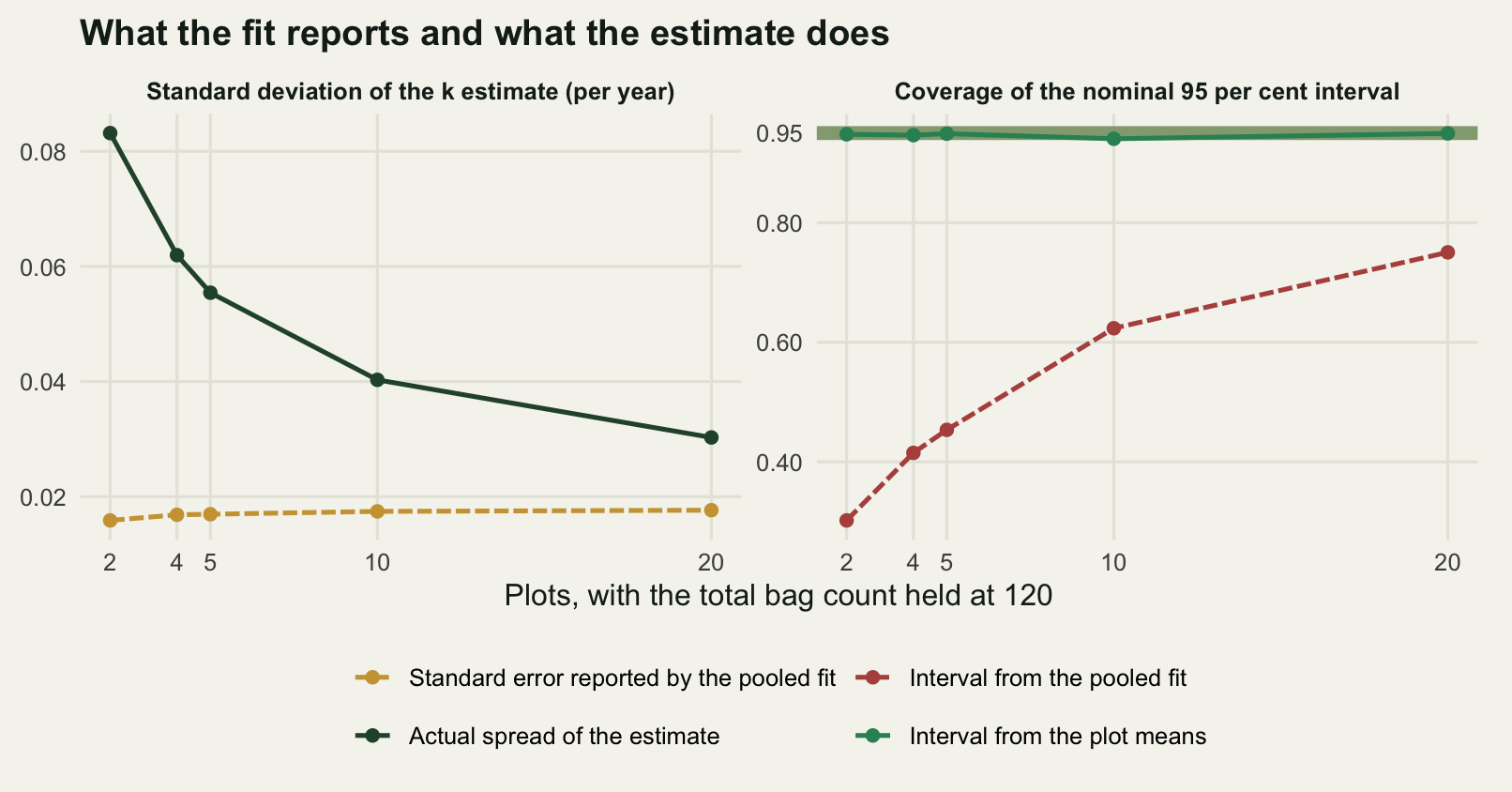
The last part of the check is a design statement, and the sweep has already made it. Holding the budget at one hundred and twenty bags, four plots with five bags per harvest gives the estimate a standard deviation of 0.0620, and twenty plots with one bag per harvest gives 0.0303. In variance that is a factor of 4.1832 for the same number of bags, the same number of harvests and the same amount of drying-oven time. Extra bags in a plot you already have buy almost nothing, because they are all measuring the same plot. The cost of a plot is walking to it. That is the trade the design has to make, and it should be made before the bags are filled, not after.
Check 2: comparing k between two treatments
The single decay constant is rarely the point. The point is that the thinned plots decompose faster than the controls, and there are three common routes to that claim.
The first fits k in every plot, as check 1 recommends, and runs a two-sample t-test on the ten plot-level estimates from each treatment. The second fits one model to all the bags with a time-by-treatment interaction on the log scale, which is what lm(log(mass) ~ 0 + time + time:treat) gives, and tests the interaction coefficient. The third fits the two treatments separately, prints their confidence intervals, and calls the difference real when the intervals do not overlap.
These are not the same test, and the sweep below measures each one over a range of true differences in k, from none at all up to 0.28 per year. At a difference of zero the rejection rate is the type I error.
set.seed(20260727)
P <- 10
nb <- 2
tp <- rep(harvest, each = nb)
np <- length(tp)
N1 <- P * np
tv1 <- rep(tp, P)
pid <- rep(seq_len(P), each = np)
S1 <- sum(tv1^2)

one_arm <- function(k) {
  u <- rnorm(P, 0, tau_plot)
  y <- -(k + u[pid]) * tv1 + rnorm(N1, 0, sig_bag)
  kh <- fit_origin(y, tv1)
  kps <- as.numeric(tapply(seq_len(N1), pid,
                           function(j) fit_origin(y[j], tv1[j])))
  list(k = kh, rss = sum((y + kh * tv1)^2), kp = kps)
}

stats_at <- function(d, R) {
  tc_sep <- qt(0.975, N1 - 1)
  out <- matrix(0, R, 3)
  for (i in seq_len(R)) {
    A <- one_arm(k_true)
    B <- one_arm(k_true - d)
    sp <- sqrt((var(A$kp) + var(B$kp)) / 2)
    out[i, 1] <- abs(mean(A$kp) - mean(B$kp)) / (sp * sqrt(2 / P))
    s2 <- (A$rss + B$rss) / (2 * N1 - 2)
    out[i, 2] <- abs(A$k - B$k) / sqrt(2 * s2 / S1)
    hA <- tc_sep * sqrt(A$rss / (N1 - 1) / S1)
    hB <- tc_sep * sqrt(B$rss / (N1 - 1) / S1)
    out[i, 3] <- abs(A$k - B$k) - (hA + hB)
  }
  out
}

diffs <- seq(0, 0.28, by = 0.04)
S <- lapply(diffs, stats_at, R = n_rep)
routes <- c("Plot-level t-test", "Interaction on all bags", "Intervals do not overlap")
nominal <- c(qt(0.975, 2 * P - 2), qt(0.975, 2 * N1 - 2), 0)
calibrated <- apply(S[[1]], 2, quantile, 0.95)
raw <- t(sapply(S, function(m) colMeans(sweep(m, 2, nominal, ">"))))
adj <- t(sapply(S, function(m) colMeans(sweep(m, 2, calibrated, ">"))))
colnames(raw) <- colnames(adj) <- routes
rownames(raw) <- rownames(adj) <- sprintf("%.2f", diffs)

print(c(plots_per_treatment = P, bags_per_treatment = N1))
plots_per_treatment bags_per_treatment
10 120 print(round(rbind(nominal_critical_value = nominal,
calibrated_critical_value = calibrated), 4)) [,1] [,2] [,3]
nominal_critical_value 2.1009 1.9700 0.0000
calibrated_critical_value 2.0801 4.5962 0.0436cat("rejection rate at the stated 5 per cent level\n")rejection rate at the stated 5 per cent levelprint(round(raw, 4)) Plot-level t-test Interaction on all bags Intervals do not overlap
0.00 0.0485 0.3905 0.2385
0.04 0.1035 0.5080 0.3370
0.08 0.2610 0.7170 0.5845
0.12 0.5000 0.8930 0.8065
0.16 0.7430 0.9775 0.9415
0.20 0.9080 0.9950 0.9870
0.24 0.9725 0.9995 0.9985
0.28 0.9970 1.0000 1.0000cat("rejection rate after each route is calibrated to 5 per cent\n")rejection rate after each route is calibrated to 5 per centprint(round(adj, 4)) Plot-level t-test Interaction on all bags Intervals do not overlap
0.00 0.0500 0.0500 0.0500
0.04 0.1105 0.1070 0.1105
0.08 0.2695 0.2790 0.2795
0.12 0.5095 0.5315 0.5375
0.16 0.7490 0.7860 0.7930
0.20 0.9110 0.9275 0.9280
0.24 0.9740 0.9790 0.9805
0.28 0.9970 0.9980 0.9985print(round(c(power_the_correct_route_gives_up_in_points =
100 * (adj["0.16", 3] - adj["0.16", 1])), 4))power_the_correct_route_gives_up_in_points
4.4 The first row of the first table is the whole check. With no difference at all between the treatments, the plot-level t-test rejects in 4.9 per cent of studies, which is the advertised rate. The interaction model on all two hundred and forty bags rejects in 39.1 per cent. The non-overlapping intervals rule rejects in 23.8 per cent.
Both of the wrong routes are wrong for the reason check 1 gave: they divide by a standard error computed between bags. The interval rule is the less bad of the two, and the reason is worth knowing, because it is not that the rule is more careful. Requiring two ninety five per cent intervals to clear each other is a stricter demand than requiring a test of the difference to reach five per cent, by roughly a factor of the square root of two on the scale of the statistic, so the interval rule is conservative when the standard errors are right. Here the standard errors are too small by a factor of 2.3091, and the two errors partly cancel. Partly. Roughly a quarter of null studies still come out significant, and the analyst has no way to tell which failure mode produced it.
Now power, at a real difference. Twenty per cent of k is 0.16 per year, which is the kind of effect a litterbag experiment is designed around. There the plot-level test rejects in 74.3 per cent of studies, the interaction model in 97.8 per cent, and the interval rule in 94.2 per cent.
That comparison is not fair and should not be read as one. A route that rejects 39.1 per cent of null studies is not a five per cent test, so its higher rejection rate under an alternative is not power in the sense anyone means. The second table fixes that by finding, for each route, the critical value that gives exactly five per cent under the null, and re-running the sweep with it.
mk_long <- function(m, lab) {
  data.frame(difference = rep(diffs, length(routes)),
             rate = as.vector(m),
             route = factor(rep(routes, each = length(diffs)), levels = routes),
             panel = lab)
}
pw <- rbind(mk_long(raw, "As each route states its level"),
            mk_long(adj, "Calibrated to 5 per cent under the null"))
pw$panel <- factor(pw$panel, levels = c("As each route states its level",
                                        "Calibrated to 5 per cent under the null"))

ggplot(pw, aes(difference, rate, colour = route, linetype = route)) +
  geom_hline(yintercept = 0.05, colour = te_pal$ink, linetype = "22",
             linewidth = 0.5) +
  geom_line(linewidth = 0.9) +
  geom_point(size = 1.8) +
  facet_wrap(~panel) +
  scale_colour_manual(values = c(te_pal$forest, te_pal$clay, te_pal$gold),
                      name = NULL) +
  scale_linetype_manual(values = c("solid", "31", "42"), name = NULL) +
  scale_y_continuous(limits = c(0, 1)) +
  guides(colour = guide_legend(nrow = 1), linetype = guide_legend(nrow = 1)) +
  labs(x = "True difference in k (per year)", y = "Rejection rate",
       title = "Three routes to one comparison") +
  theme_te() +
  theme(strip.text = element_text(colour = te_pal$ink, face = "bold"),
        legend.text = element_text(size = 9),
        plot.margin = margin(8, 14, 8, 8))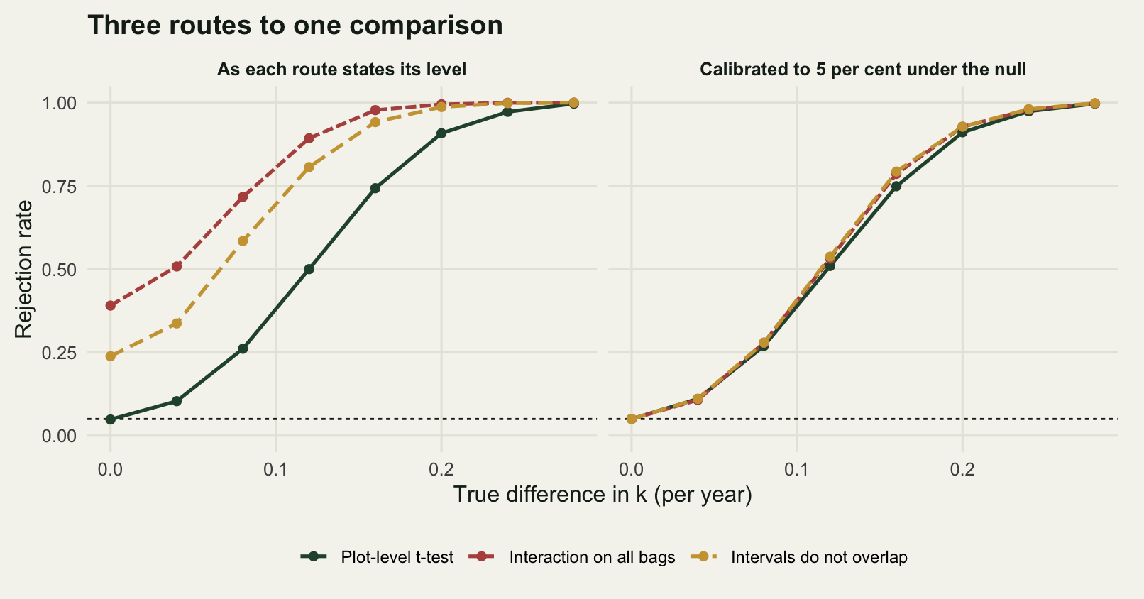
The second panel is the useful part. Once every route is calibrated to the same size, they are nearly equally sensitive: at a difference of 0.16 the three give 74.9, 78.6 and 79.3 per cent. The correct route is the lowest of the three, which it also is before calibration, but the gap has closed to a few percentage points. It pays about 4.4 percentage points of power for estimating the between-plot variance from ten plots instead of assuming it away.
So the objection to the bag-level routes is not that they are insensitive. They are slightly the more sensitive statistics. The objection is that the number printed next to them is not the error rate they have, and nothing in the output says so. A calibrated bag-level test is a fine test and nobody runs one, because the calibration requires knowing the between-plot variance, which is what the plot-level route estimates directly.
The late harvests are noisier, and unweighted fits do not know
There is a second problem in the comparison, and it lives in the variance rather than the mean. Part of the error on a litterbag is a fixed quantity of mass: a balance error, a gram of soil that would not brush off, a few roots missed in the picking. A fixed error in grams is a small relative error on a bag holding most of its mass and a large one on a bag holding a tenth of it, so on the log scale the variance grows as the study runs.
The sub-check below adds an additive component of 0.025 of initial mass to the multiplicative one and extends the schedule to three years, where the last bags are down near a tenth. Plot-level variation is switched off so that the only defect left is the variance function. Working on the log scale needs the additive component expressed there, and to first order it contributes a standard deviation of the additive error divided by the mean mass remaining. The first chunk output checks that approximation against the exact additive generator before anything is built on it.
set.seed(20260728)
sig_add <- 0.025
har3 <- c(0.25, 0.5, 0.75, 1, 1.5, 2, 3)
nb3 <- 6

s_of_t <- function(t) sqrt(sig_bag^2 + (sig_add / exp(-k_true * t))^2)
calib <- sapply(har3, function(tt) {
  m <- exp(-k_true * tt)
  yy <- m * exp(rnorm(60000, 0, sig_bag)) + rnorm(60000, 0, sig_add)
  c(exact_sd = sd(log(yy[yy > 0])), first_order_sd = s_of_t(tt),
    share_of_bags_at_or_below_zero = mean(yy <= 0))
})
colnames(calib) <- har3
print(round(calib, 5))
0.25 0.5 0.75 1 1.5 2
exact_sd 0.18371 0.18439 0.18700 0.18993 0.20205 0.22557
first_order_sd 0.18257 0.18382 0.18567 0.18840 0.19822 0.21848
share_of_bags_at_or_below_zero 0.00000 0.00000 0.00000 0.00000 0.00000 0.00000
3
exact_sd 0.38833
first_order_sd 0.32916
share_of_bags_at_or_below_zero 0.00063print(round(c(first_order_shortfall_at_three_years_percent =
100 * (1 - calib["first_order_sd", "3"] /
calib["exact_sd", "3"])), 4))first_order_shortfall_at_three_years_percent
15.2388 tv3 <- rep(har3, each = nb3)
zz <- rep(0:1, each = length(tv3))
tt3 <- rep(tv3, 2)
ss3 <- s_of_t(tt3)
X <- cbind(tt3, tt3 * zz)
Nh <- length(tt3)
W <- 1 / ss3^2
XtXi <- solve(crossprod(X))
XtWXi <- solve(t(X) %*% (W * X))
tc3 <- qt(0.975, Nh - 2)
ok_o <- ok_w <- bo_v <- bw_v <- numeric(n_rep)
for (i in seq_len(n_rep)) {
ly <- -k_true * tt3 + rnorm(Nh, 0, ss3)
bo <- XtXi %*% crossprod(X, ly)
ro <- ly - X %*% bo
seo <- sqrt(sum(ro^2) / (Nh - 2) * XtXi[2, 2])
bw <- XtWXi %*% (t(X) %*% (W * ly))
rw <- ly - X %*% bw
sew <- sqrt(sum(W * rw^2) / (Nh - 2) * XtWXi[2, 2])
ok_o[i] <- abs(bo[2]) <= tc3 * seo
ok_w[i] <- abs(bw[2]) <= tc3 * sew
bo_v[i] <- bo[2]
bw_v[i] <- bw[2]
}
het <- c(bags_per_treatment = length(tv3),
variance_ratio_last_over_first =
s_of_t(max(har3))^2 / s_of_t(min(har3))^2,
coverage_unweighted = mean(ok_o), coverage_weighted = mean(ok_w),
sd_unweighted = sd(bo_v), sd_weighted = sd(bw_v),
extra_bags_the_unweighted_fit_needs = var(bo_v) / var(bw_v),
theory_sd_unweighted =
sqrt((XtXi %*% t(X) %*% (ss3^2 * X) %*% XtXi)[2, 2]),
theory_sd_weighted = sqrt(XtWXi[2, 2]))
print(round(het, 5)) bags_per_treatment variance_ratio_last_over_first
42.00000 3.25041
coverage_unweighted coverage_weighted
0.88200 0.95650
sd_unweighted sd_weighted
0.03784 0.03367
extra_bags_the_unweighted_fit_needs theory_sd_unweighted
1.26322 0.03873
theory_sd_weighted
0.03463 The first-order approximation holds up to about two years and then starts to run short: at the three-year harvest it gives a log-scale standard deviation of 0.32916 against 0.38833 from the exact additive generator, an underestimate of 15.2 per cent, and in that generator 0.06333 per cent of bags come back at or below zero mass, where the log does not exist. Everything below therefore understates the problem rather than overstating it.
On the log scale the variance at the last harvest is 3.2504 times the variance at the first. An unweighted fit treats those bags as equally informative, and the interval it prints for the treatment difference covers in 88.2 per cent of replicates instead of ninety five. Weighting by the inverse of the variance function restores it to 95.6 per cent, and shrinks the standard deviation of the estimate from 0.0378 to 0.0337, so the unweighted fit needs 1.2632 times as many bags to match it. The sandwich estimates from the design agree with the simulation: 0.03873 against 0.03784.
The efficiency loss is the smaller half of that. The interval is the larger half, because a coverage of 88.2 per cent is what a reader is not told about. Variance structure and heteroscedasticity sets out how to specify a variance function properly, including estimating its parameters rather than knowing them as they are known here.
Check 3: the mass that was gone before the first harvest
Every litterbag paper fixes the intercept at one. The bags started as themselves, so the curve starts at one hundred per cent.
The bags did not start as themselves. Air-dried mass is converted to oven-dried mass through a subsample and a ratio. Fragments break off in the crate on the way to the site. The finest material washes through the mesh in the first storm, which is mass loss but not decomposition. By the first harvest, weeks or months after the bags went out, the curve the data follow may start a few per cent below one, and forcing it through one tilts the whole line.
The bias that produces, and the question of whether to free the intercept instead, is worked out in fitting litter decomposition curves, which measures the root mean squared error both ways and finds that in a short study the biased fit wins. What this check adds is the diagnostic: given that almost everyone will fix the intercept, can the loss be seen in what the fit leaves behind.
Two statistics are on trial, both computed from the residuals of the fixed-intercept fit. The first is the mean residual at the earliest harvest, which is the one a reader can estimate off a published figure with a ruler. The second is the trend of the residuals against time. Plot-level variation is switched off so that the loss is the only defect present; the handling loss is 0.05 of initial mass.
set.seed(20260730)
loss <- 0.05
M0 <- 1 - loss
lev <- sum(harvest) / sum(harvest^2)

resid_stats <- function(nb, R, m0) {
  tv <- rep(harvest, each = nb)
  N <- length(tv)
  first <- tv == min(harvest)
  tbar <- mean(tv)
  Sxx <- sum((tv - tbar)^2)
  out <- matrix(0, R, 4)
  for (i in seq_len(R)) {
    ly <- log(m0) - k_true * tv + rnorm(N, 0, sig_bag)
    kh <- fit_origin(ly, tv)
    res <- ly + kh * tv
    b1 <- sum((tv - tbar) * ly) / Sxx
    out[i, ] <- c(mean(res[first]),
                  sum((tv - tbar) * res) / Sxx,
                  mean(ly) - b1 * tbar,
                  kh)
  }
  out
}

nbs <- c(2, 4, 6, 8, 12, 20, 30)
det <- t(sapply(nbs, function(nb) {
  a <- resid_stats(nb, n_rep, 1)
  b <- resid_stats(nb, n_rep, M0)
  crit <- apply(abs(a[, 1:2]), 2, quantile, 0.95)
  c(bags_per_harvest = nb, bags = nb * length(harvest),
    detect_first_harvest_residual = mean(abs(b[, 1]) > crit[1]),
    detect_residual_trend = mean(abs(b[, 2]) > crit[2]),
    residual_at_first_harvest_correct_model = mean(a[, 1]),
    residual_at_first_harvest_with_loss = mean(b[, 1]),
    k_correct_model = mean(a[, 4]), k_with_loss = mean(b[, 4]),
    largest_gap_trend_versus_free_intercept =
      max(abs(b[, 2] + lev * b[, 3])))
}))
rownames(det) <- paste(nbs, "bags per harvest")

mean_res <- function(m0, nb, R) {
  tv <- rep(harvest, each = nb)
  tot <- numeric(length(harvest))
  for (i in seq_len(R)) {
    ly <- log(m0) - k_true * tv + rnorm(length(tv), 0, sig_bag)
    tot <- tot + as.numeric(tapply(ly + fit_origin(ly, tv) * tv, tv, mean))
  }
  tot / R
}
n_res <- 800
res_by_harvest <- rbind(correct_model = mean_res(1, 8, n_res),
                        with_handling_loss = mean_res(M0, 8, n_res),
                        closed_form = log(M0) * (1 - lev * harvest))
colnames(res_by_harvest) <- harvest

print(round(det[, 1:6], 5))
bags_per_harvest bags detect_first_harvest_residual
2 bags per harvest 2 12 0.0810
4 bags per harvest 4 24 0.0695
6 bags per harvest 6 36 0.0835
8 bags per harvest 8 48 0.1140
12 bags per harvest 12 72 0.1075
20 bags per harvest 20 120 0.1640
30 bags per harvest 30 180 0.2435
detect_residual_trend
2 bags per harvest 0.0880
4 bags per harvest 0.1010
6 bags per harvest 0.1485
8 bags per harvest 0.1680
12 bags per harvest 0.2105
20 bags per harvest 0.3405
30 bags per harvest 0.5190
residual_at_first_harvest_correct_model
2 bags per harvest -0.00176
4 bags per harvest -0.00413
6 bags per harvest -0.00260
8 bags per harvest -0.00040
12 bags per harvest 0.00042
20 bags per harvest 0.00256
30 bags per harvest -0.00031
residual_at_first_harvest_with_loss
2 bags per harvest -0.04444
4 bags per harvest -0.04187
6 bags per harvest -0.04070
8 bags per harvest -0.04228
12 bags per harvest -0.04013
20 bags per harvest -0.04252
30 bags per harvest -0.04240print(round(det[, c(1, 7, 8, 9)], 6)) bags_per_harvest k_correct_model k_with_loss
2 bags per harvest 2 0.800748 0.838500
4 bags per harvest 4 0.798465 0.837662
6 bags per harvest 6 0.799797 0.838136
8 bags per harvest 8 0.800097 0.839092
12 bags per harvest 12 0.799623 0.837777
20 bags per harvest 20 0.799496 0.837368
30 bags per harvest 30 0.800302 0.837575
largest_gap_trend_versus_free_intercept
2 bags per harvest 0
4 bags per harvest 0
6 bags per harvest 0
8 bags per harvest 0
12 bags per harvest 0
20 bags per harvest 0
30 bags per harvest 0print(c(replicates_per_residual_curve = n_res))replicates_per_residual_curve
800 print(round(res_by_harvest, 5)) 0.25 0.5 0.75 1 1.5 2
correct_model 0.00247 0.00147 -0.00136 0.00051 -0.00244 0.00141
with_handling_loss -0.04315 -0.03301 -0.02241 -0.01547 0.00923 0.02286
closed_form -0.04182 -0.03235 -0.02288 -0.01342 0.00552 0.02446print(round(c(k_bias_at_eight_bags_per_harvest =
det["8 bags per harvest", "k_with_loss"] - k_true,
k_bias_percent =
100 * (det["8 bags per harvest", "k_with_loss"] - k_true) / k_true), 5))k_bias_at_eight_bags_per_harvest k_bias_percent
0.03909 4.88656 print(round(c(handling_loss = loss, true_intercept = M0,
bias_formula = -log(M0) * lev,
theoretical_first_harvest_residual =
log(M0) * (1 - lev * min(harvest)),
theoretical_last_harvest_residual =
log(M0) * (1 - lev * max(harvest))), 5)) handling_loss true_intercept
0.05000 0.95000
bias_formula theoretical_first_harvest_residual
0.03788 -0.04182
theoretical_last_harvest_residual
0.02446 Start with what the loss does to k. Fixing the intercept at one when the litter started at 0.95 steepens the fit: the estimate goes from 0.8001 under the correct model to 0.8391, a bias of 4.9 per cent. The closed form for that bias is minus the log of the intercept times the sum of the harvest times over the sum of their squares, which gives 0.03788 against a simulated 0.03909. It does not depend on how many bags there are, only on when the harvests are.
Now the residuals. Under the correct model the mean residual at the first harvest is -0.00040, which is zero to within simulation noise. Under a 5 per cent handling loss it is -0.04228, against a theoretical -0.04182. The residual at the last harvest goes the other way, to 0.02446. The fixed line starts above the data and ends below it, which is a tilt and not a curve, and that is what makes it hard to see: a tilt looks like scatter unless you know where the line should have been.
The detection columns say how hard. With eight bags per harvest, forty eight bags in all, the first harvest residual detects the loss in 11.4 per cent of studies against a five per cent null rate, and the residual trend in 16.8 per cent. At thirty bags per harvest, one hundred and eighty bags, they reach 24.3 and 51.9 per cent.
tgrid <- seq(0, max(harvest), length.out = 121)
res_line <- rbind(
  data.frame(t = tgrid, value = 0, series = "Correct model"),
  data.frame(t = tgrid, value = log(M0) * (1 - lev * tgrid),
             series = "5 per cent handling loss"))
res_line$panel <- "Mean residual, by harvest time in years"
res_pt <- rbind(
  data.frame(t = harvest, value = res_by_harvest["correct_model", ],
             series = "Correct model"),
  data.frame(t = harvest, value = res_by_harvest["with_handling_loss", ],
             series = "5 per cent handling loss"))
res_pt$panel <- "Mean residual, by harvest time in years"

dd <- as.data.frame(det)
det_df <- rbind(
  data.frame(t = dd$bags_per_harvest, value = dd$detect_first_harvest_residual,
             series = "Residual at the first harvest"),
  data.frame(t = dd$bags_per_harvest, value = dd$detect_residual_trend,
             series = "Trend of the residuals on time"))
det_df$panel <- "Detection probability, by bags per harvest"

lv3 <- c("Correct model", "5 per cent handling loss",
         "Residual at the first harvest", "Trend of the residuals on time")
pn3 <- c("Mean residual, by harvest time in years",
         "Detection probability, by bags per harvest")
for (D in c("res_line", "res_pt", "det_df")) {
  x <- get(D)
  x$series <- factor(x$series, levels = lv3)
  x$panel <- factor(x$panel, levels = pn3)
  assign(D, x)
}
ref3 <- data.frame(panel = factor(pn3[2], levels = pn3), y = 0.05)
tags <- data.frame(
  t = c(0.12, 0.12, 2.6, 2.6),
  value = c(0.0195, 0.0055, 0.48, 0.425),
  lab = lv3[c(2, 1, 4, 3)],
  series = factor(lv3[c(2, 1, 4, 3)], levels = lv3),
  panel = factor(pn3[c(1, 1, 2, 2)], levels = pn3))

ggplot(mapping = aes(t, value, colour = series, linetype = series)) +
  geom_hline(data = ref3, aes(yintercept = y),
             colour = te_pal$ink, linetype = "22", linewidth = 0.5) +
  geom_line(data = res_line, linewidth = 0.9) +
  geom_point(data = res_pt, aes(shape = series), size = 2.2) +
  geom_line(data = det_df, linewidth = 0.9) +
  geom_point(data = det_df, aes(shape = series), size = 2.2) +
  geom_text(data = tags, aes(label = lab), hjust = 0, size = 3.1,
            show.legend = FALSE) +
  facet_wrap(~panel, scales = "free") +
  scale_colour_manual(values = c(te_pal$forest, te_pal$clay,
                                 te_pal$green, te_pal$gold), name = NULL) +
  scale_linetype_manual(values = c("solid", "31", "solid", "42"), name = NULL) +
  scale_shape_manual(values = c(16, 17, 15, 18), name = NULL) +
  labs(x = NULL, y = NULL,
       title = "A tilt in the residuals, and how often anyone sees it") +
  theme_te() +
  theme(strip.text = element_text(colour = te_pal$ink, face = "bold"),
        legend.position = "none",
        plot.margin = margin(8, 14, 8, 8))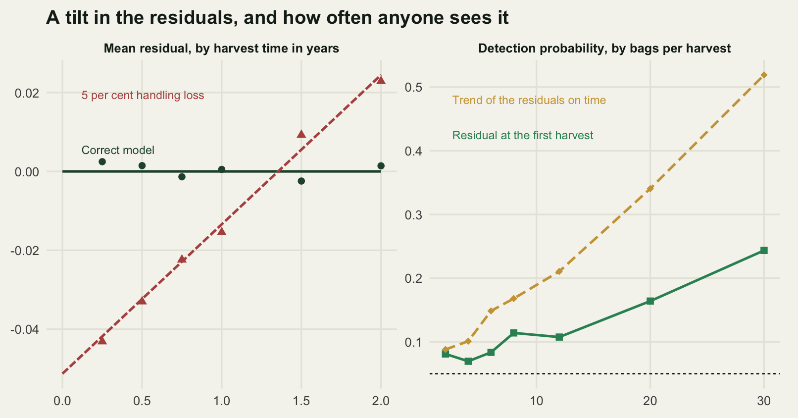
Two things fall out of that, and one of them was not what I expected when I set the check up.
The first is that the residual trend statistic is not a new test. It is the free-intercept fit written a different way: the trend of the residuals from a through-origin fit is exactly minus the free-intercept estimate times the sum of the harvest times over the sum of their squares. The largest disagreement between the two over 2000 replicates is 0.000000. So the choice is not between a residual check and a proper test. It is between the whole residual pattern, which is the proper test, and the first point of it, which is not.
The second is that neither of them works. At the design in this post, a five per cent handling loss is caught about one time in six by the stronger of the two statistics, and even the largest design in the sweep takes it only to a bare one in two. That is a real limit on what a diagnostic can do, and it points at a field procedure rather than a statistical one: weigh a set of bags, take them to the site, bring them straight back, and weigh them again. Ten bags treated that way measure the handling loss directly and settle in an afternoon a question that a hundred and eighty buried bags cannot settle in two years.
The first-harvest residual is still worth computing, for one reason: it is the only one of the two that a reader can run on somebody else’s published figure. It catches the loss 11.4 per cent of the time on a forty eight bag study, which is not much, but it costs nothing and the alternative is assuming the intercept was right.
Check 4: the number that sits outside the data
The quantities that leave a decomposition paper are usually not the ones the bags measured. A two-year study reports an annual k. A nine-month study reports a mean residence time. Almost everybody reports a time to ninety five per cent mass loss, which for these litters is years past the last bag anyone lifted.
The check has two halves. First, does the fitted model predict data it has not seen: refit on the early harvests and predict the late ones, against the model’s own predictive interval. Second, how wide is the interval on the extrapolated quantity when the uncertainty is propagated honestly.
To make the check able to fail, the truth here is two pools rather than one, with a labile fraction of 0.7 decaying at 1.6 per year and the rest at 0.15. That is ordinary litter. Nothing else about the study changes.
set.seed(20260731)
lab_frac <- 0.7
k_fast <- 1.6
k_slow <- 0.15
two_pool <- function(t) lab_frac * exp(-k_fast * t) + (1 - lab_frac) * exp(-k_slow * t)
target <- 0.05
t95 <- function(k) -log(target) / k
t95_true <- uniroot(function(t) two_pool(t) - target, c(0.1, 200), tol = 1e-10)$root

k_win <- function(w) {
  tt <- harvest[harvest <= w]
  -sum(tt * log(two_pool(tt))) / sum(tt^2)
}
wins <- c(0.75, 1, 1.5, 2)
wtab <- t(sapply(wins, function(w) c(window_end_years = w,
                                     harvests_used = sum(harvest <= w),
                                     k = k_win(w), time_to_95_percent = t95(k_win(w)))))
k_full <- k_win(max(harvest))
misfit <- log(two_pool(harvest)) + k_full * harvest

print(round(wtab, 5))
window_end_years harvests_used k time_to_95_percent
[1,] 0.75 3 1.00890 2.96931
[2,] 1.00 4 0.96012 3.12016
[3,] 1.50 5 0.87054 3.44124
[4,] 2.00 6 0.78244 3.82869print(round(c(true_time_to_95_percent = t95_true,
largest_misfit_in_bag_sds = max(abs(misfit)) / sig_bag,
largest_misfit_in_harvest_mean_sds =
max(abs(misfit)) / (sig_bag / sqrt(P * nb))), 4)) true_time_to_95_percent largest_misfit_in_bag_sds
11.9451 1.0095
largest_misfit_in_harvest_mean_sds
4.5144 kh <- se_pool <- se_plot <- numeric(n_rep)
for (i in seq_len(n_rep)) {
u <- rnorm(P, 0, tau_plot)
ly <- log(two_pool(tv1)) - u[pid] * tv1 + rnorm(N1, 0, sig_bag)
k <- fit_origin(ly, tv1)
kh[i] <- k
se_pool[i] <- sqrt(sum((ly + k * tv1)^2) / (N1 - 1) / S1)
kps <- as.numeric(tapply(seq_len(N1), pid,
function(j) fit_origin(ly[j], tv1[j])))
se_plot[i] <- sd(kps) / sqrt(P)
}
tc_a <- qt(0.975, N1 - 1)
tc_b <- qt(0.975, P - 1)
w_paper <- mean(t95(kh - tc_a * se_pool) - t95(kh + tc_a * se_pool))
w_honest <- mean(t95(kh - tc_b * se_plot) - t95(kh + tc_b * se_plot))
ex <- c(fitted_k = mean(kh), fitted_time_to_95_percent = mean(t95(kh)),
simulated_sd_of_the_estimate = sd(t95(kh)),
delta_method_sd = mean(-log(target) * se_plot / kh^2),
width_from_the_pooled_se = w_paper,
width_with_plots_propagated = w_honest,
honest_over_quoted = w_honest / w_paper,
error_in_years = t95_true - mean(t95(kh)),
error_over_the_honest_width = (t95_true - mean(t95(kh))) / w_honest,
error_over_the_quoted_width = (t95_true - mean(t95(kh))) / w_paper)
print(round(ex, 5)) fitted_k fitted_time_to_95_percent
0.78326 3.83551
simulated_sd_of_the_estimate delta_method_sd
0.20495 0.19446
width_from_the_pooled_se width_with_plots_propagated
0.39531 0.89367
honest_over_quoted error_in_years
2.26070 8.10955
error_over_the_honest_width error_over_the_quoted_width
9.07440 20.51445 The nested windows come first because they need no simulation at all, only the noiseless curve. Fit the single exponential to the first three harvests and it gives 1.0089; to four harvests, 0.9601; to five, 0.8705; to all six, 0.7824. The time to ninety five per cent loss moves with it, from 2.9693 years to 3.8287. That drift has a direction, and the direction is the whole signal: every extra harvest makes the extrapolated time longer, so the sequence has not converged and the last value is not the limit, only the largest one so far. The true answer for this litter is 11.9451 years.
Nobody notices, because the single exponential fits the data. Its largest departure from the two-pool curve inside the two-year window is 1.0095 bag standard deviations, which is invisible in a scatter of individual bags. Plot harvest means instead and the same departure is 4.5144 standard errors, which is not invisible at all. That is a free check and the reason to draw the mean of each harvest as well as the bags.
Now the intervals. Fitted on the full two years, the study returns 0.7833 for k and 3.8355 years for the time to ninety five per cent loss. The interval a paper would quote, propagating the standard error the pooled fit prints, is 0.3953 years wide. Propagating the plot-level standard error from check 1 instead gives 0.8937 years, which is 2.2607 times wider. Simulating the estimate from the parameter distribution and taking its spread gives 0.20495, against 0.19446 from the delta method, so for a quantity this simple the two agree and the delta method is not the problem.
The problem is that both intervals are answers to a question about k, and the reported quantity is not a question about k. The error here is 8.1096 years, which is 9.0744 times the honest interval and 20.5144 times the quoted one. No amount of care with the standard error reaches it, because the missing term is the model, and a confidence interval conditions on the model being right.
set.seed(20260801)
early <- harvest[harvest <= 0.75]
late <- harvest[harvest > 0.75]
n_per <- P * nb
tv_e <- rep(early, each = n_per)

pred_check <- function(gen, R) {
  hit <- z <- matrix(0, R, length(late))
  for (i in seq_len(R)) {
    ly <- gen(tv_e) + rnorm(length(tv_e), 0, sig_bag)
    k <- fit_origin(ly, tv_e)
    s2 <- sum((ly + k * tv_e)^2) / (length(tv_e) - 1)
    vk <- s2 / sum(tv_e^2)
    for (j in seq_along(late)) {
      obs <- mean(gen(rep(late[j], n_per)) + rnorm(n_per, 0, sig_bag))
      sp <- sqrt(late[j]^2 * vk + s2 / n_per)
      z[i, j] <- (obs + k * late[j]) / sp
      hit[i, j] <- abs(z[i, j]) <= qt(0.975, length(tv_e) - 1)
    }
  }
  rbind(coverage = colMeans(hit), mean_standardised_error = colMeans(z))
}
n_pred <- 800
print(c(replicates = n_pred, bags_per_harvest = n_per,
        harvests_fitted = length(early), harvests_held_out = length(late)))
replicates bags_per_harvest harvests_fitted harvests_held_out
800 20 3 3 one_exp <- pred_check(function(t) -k_true * t, n_pred)
two_p <- pred_check(function(t) log(two_pool(t)), n_pred)
colnames(one_exp) <- colnames(two_p) <- late
cat("truth is a single exponential\n")truth is a single exponentialprint(round(one_exp, 4)) 1 1.5 2
coverage 0.9425 0.9488 0.9612
mean_standardised_error -0.0173 -0.0559 0.0008cat("truth is two pools\n")truth is two poolsprint(round(two_p, 4)) 1 1.5 2
coverage 0.6838 0.0150 0.0000
mean_standardised_error 1.5612 4.1752 6.6974The single-exponential run is the calibration. When the model is right, the interval built from the first three harvests contains the mean of each held-out harvest 94.2, 94.9 and 96.1 per cent of the time, which is what ninety five per cent should look like, so the machinery is not the thing that fails next.
On two-pool litter it fails completely. Coverage at one year is 68.4 per cent, at one and a half years 1.5 per cent, and at two years 0.0 per cent. The standardised prediction error grows from 1.5612 to 6.6974 predictive standard deviations, all in the same direction: the bags hold more mass than the early fit says they should, because the labile pool has gone and the fit does not know there is a slower one behind it.
k_early <- k_win(0.75)
s2_e <- sig_bag^2
vk_e <- s2_e / sum(tv_e^2)
tq <- qt(0.975, length(tv_e) - 1)
gl <- seq(0.05, 2, length.out = 200)
band <- data.frame(
  t = gl,
  fit = exp(-k_early * gl),
  lo = exp(-k_early * gl - tq * sqrt(gl^2 * vk_e + s2_e / n_per)),
  hi = exp(-k_early * gl + tq * sqrt(gl^2 * vk_e + s2_e / n_per)),
  panel = "The harvests held out of the fit")
obs_pt <- data.frame(t = harvest, mass = two_pool(harvest),
                     role = ifelse(harvest <= 0.75, "Harvests used in the fit",
                                   "Harvests held out"),
                     panel = "The harvests held out of the fit")
gr <- seq(0, 13, length.out = 1301)
curves <- rbind(
  data.frame(t = gr, mass = two_pool(gr), series = "Two pool truth"),
  data.frame(t = gr, mass = exp(-ex[["fitted_k"]] * gr),
             series = "Fitted single exponential"))
curves <- curves[curves$mass <= 0.30, ]
curves$panel <- "Time to 95 per cent mass loss"
half <- c(ex[["width_with_plots_propagated"]], ex[["width_from_the_pooled_se"]]) / 2
bands <- data.frame(
  x0 = ex[["fitted_time_to_95_percent"]] - half,
  x1 = ex[["fitted_time_to_95_percent"]] + half,
  shade = c(te_pal$sage, te_pal$gold),
  panel = "Time to 95 per cent mass loss")
band_lab <- data.frame(
  t = ex[["fitted_time_to_95_percent"]] + half[1] + 0.2,
  mass = c(0.245, 0.212),
  lab = c("wide band: plots propagated",
          "narrow band: pooled standard error"),
  panel = "Time to 95 per cent mass loss")
note <- data.frame(
  t = 1.15,
  mass = 0.88 * exp(-k_early * 1.15 - tq * sqrt(1.15^2 * vk_e + s2_e / n_per)),
  lab = "fit on the first three harvests",
  panel = "The harvests held out of the fit")
pn4 <- c("The harvests held out of the fit", "Time to 95 per cent mass loss")
for (D in c("band", "obs_pt", "curves", "bands", "band_lab", "note")) {
  x <- get(D)
  x$panel <- factor(x$panel, levels = pn4)
  assign(D, x)
}
hl <- data.frame(panel = factor(pn4[2], levels = pn4), y = target)
vl <- data.frame(panel = factor(pn4[2], levels = pn4), x = t95_true)

ggplot(mapping = aes(t, mass)) +
  geom_rect(data = bands, inherit.aes = FALSE,
            mapping = aes(xmin = x0, xmax = x1, ymin = -Inf, ymax = Inf),
            fill = bands$shade, alpha = 0.5) +
  geom_ribbon(data = band, mapping = aes(x = t, ymin = lo, ymax = hi),
              inherit.aes = FALSE, fill = te_pal$sage, alpha = 0.35) +
  geom_line(data = band, mapping = aes(t, fit), colour = te_pal$forest,
            linewidth = 0.9) +
  geom_text(data = note, mapping = aes(t, mass, label = lab), hjust = 1,
            vjust = 1, size = 3, colour = te_pal$ink) +
  geom_point(data = obs_pt, mapping = aes(t, mass, shape = role), size = 2.6,
             colour = te_pal$ink) +
  geom_hline(data = hl, aes(yintercept = y),
             colour = te_pal$ink, linetype = "12", linewidth = 0.5) +
  geom_vline(data = vl, aes(xintercept = x),
             colour = te_pal$ink, linetype = "22", linewidth = 0.5) +
  geom_line(data = curves, mapping = aes(t, mass, colour = series,
                                         linetype = series), linewidth = 0.9) +
  geom_text(data = band_lab, inherit.aes = FALSE,
            mapping = aes(x = t, y = mass, label = lab),
            hjust = 0, size = 3, colour = te_pal$ink) +
  geom_text(data = vl, inherit.aes = FALSE,
            mapping = aes(x = x - 0.35, y = 0.275), label = "true value",
            hjust = 1, size = 3.2, colour = te_pal$ink) +
  facet_wrap(~panel, scales = "free") +
  scale_colour_manual(values = c(te_pal$forest, te_pal$clay), name = NULL) +
  scale_linetype_manual(values = c("solid", "31"), name = NULL) +
  scale_shape_manual(values = c(2, 16), name = NULL) +
  guides(colour = guide_legend(order = 1), linetype = guide_legend(order = 1),
         shape = guide_legend(order = 2)) +
  labs(x = "Years", y = "Mass remaining (proportion of initial)",
       title = "Predicting what was held out, and what was never measured") +
  theme_te() +
  theme(strip.text = element_text(colour = te_pal$ink, face = "bold"),
        legend.text = element_text(size = 9),
        plot.margin = margin(8, 16, 8, 8))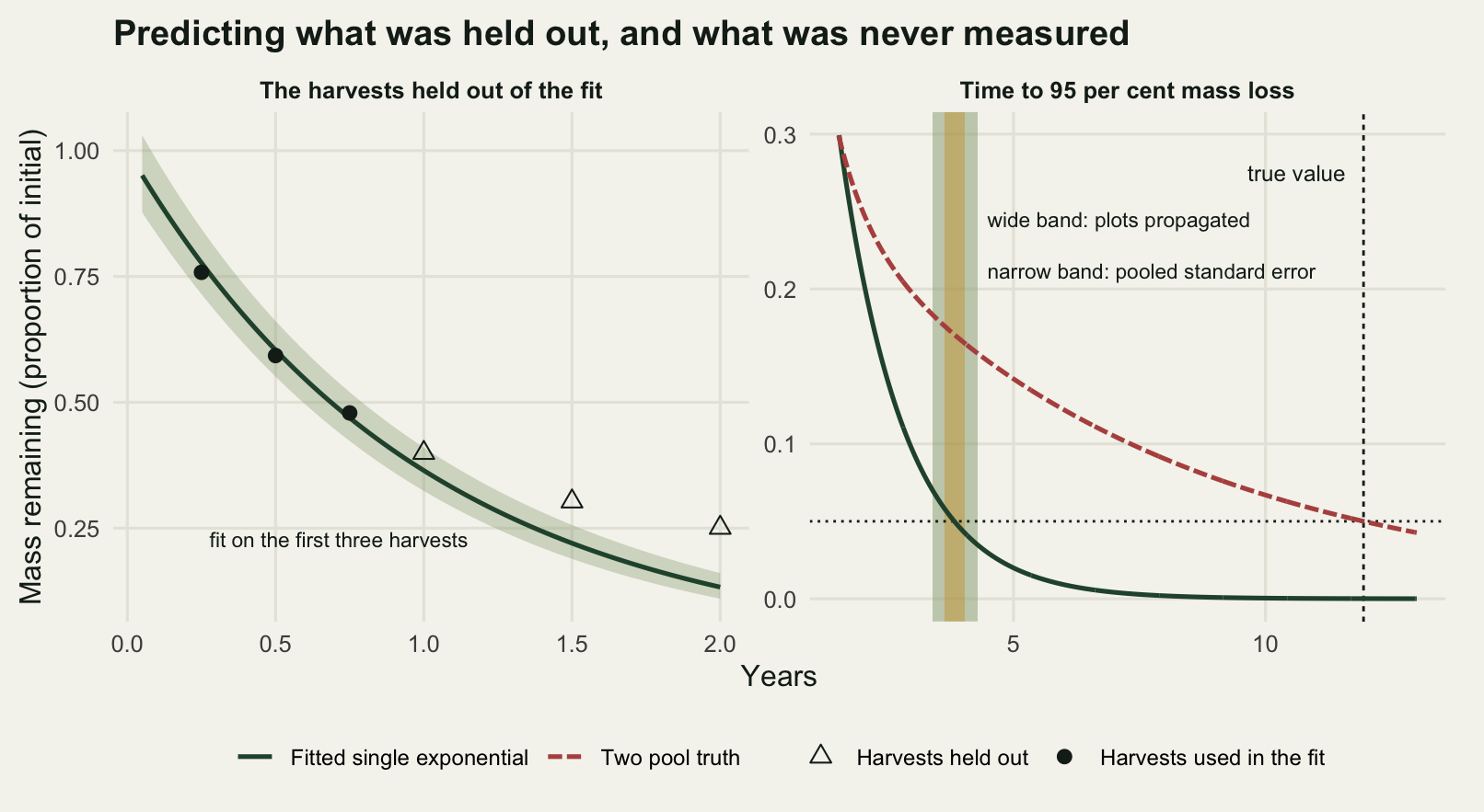
The honest limit
The four checks catch four different failures and they do not substitute for one another. Check 1 catches an interval that is too narrow, and leaves the point estimate alone. Check 2 catches a comparison whose stated error rate is not its error rate, and it is the only one of the four that changes whether a paper has a result. Check 3 catches litter that was already lighter than it was weighed at, and it catches it badly. Check 4 catches an extrapolation, and it is the only one that can move a number by a factor rather than a few per cent.
Check 3 is the weak one and the post has already said so. A five per cent handling loss is found about one study in six at forty eight bags and about one in two at one hundred and eighty. Reporting it as a check is honest only if the failure to detect is reported with it, because a residual plot that shows nothing is not evidence that nothing is there.
The larger limit is what all four have in common. Every one of them tests the estimator or the design: whether the standard error matches the randomisation, whether the test has its stated size, whether the intercept was where it was assumed to be, whether the fitted curve reaches the number being quoted. None of them tests whether the litterbag was measuring the quantity anyone needed. Mesh size sets which decomposers get in. Bags change the moisture regime of the litter inside them. Fragmented material leaves through the mesh and is counted as mass loss when it has only moved. The carbon that leaves as dissolved organic matter and the carbon that leaves as respiration are the same mass loss to a balance and different things to a budget. A litterbag study that is measuring none of what the budget needs will pass all four checks in this post, with a clean residual plot, a correctly sized test and an honest interval around a quantity that does not answer the question. That half of the problem is measured in mass loss and the carbon budget.
Three narrower limits are worth stating. The plot-level fix in check 1 works because the design is balanced; with bags lost to badgers and floods it becomes a weighted mean and the weights need thought. The variance function in check 2 is known here and would have to be estimated in practice, which costs precision that is not counted. And the two-pool truth in check 4 is itself a model, so the eight-year error it produces is a demonstration that model error can be large, not an estimate of how large it is in any particular study.
Where to go next
The cheapest of these to run on an analysis you already have is check 1, and it takes ten minutes: fit k in each plot, take the mean and the standard deviation of those numbers, and compare the result with the standard error the pooled model printed. A few per cent is the wrong trigger: the plot-level standard error is itself estimated from ten plot values, so a modest disagreement is inside its own noise. When it comes out about twice the pooled one, as it does in check 1, the pooled interval is the wrong one and every test built on it inherits the problem. The second cheapest is the window sweep in check 4, which needs no new data and no simulation: refit on the first two thirds of the harvests and see whether the quantity you plan to report moves, and in which direction.
For the machinery, checking a nonlinear model covers the diagnostics for the fit itself, which this post assumed had already passed, and power analysis by simulation is the general form of the sweep in check 2. When the quantity of interest is a function of the parameters, as the time to ninety five per cent loss is, bootstrap confidence intervals is the route that does not need the delta method to hold. And if the same bags are weighed repeatedly rather than harvested destructively, the plot term here becomes a within-bag correlation over time, which is repeated measures and temporal correlation.
References
Olson JS 1963 Ecology 44(2):322-331 (10.2307/1932179)
Hurlbert SH 1984 Ecological Monographs 54(2):187-211 (10.2307/1942661)
Bolker BM, Brooks ME, Clark CJ, Geange SW, Poulsen JR, Stevens MHH, White JSS 2009 Trends in Ecology and Evolution 24(3):127-135 (10.1016/j.tree.2008.10.008)
Zuur AF, Ieno EN, Elphick CS 2010 Methods in Ecology and Evolution 1(1):3-14 (10.1111/j.2041-210X.2009.00001.x)
Adair EC, Parton WJ, Del Grosso SJ, Silver WL, Harmon ME, Hall SA, Burke IC, Hart SC 2008 Global Change Biology 14(11):2636-2660 (10.1111/j.1365-2486.2008.01674.x)
Cornwell WK, Weedon JT 2014 Methods in Ecology and Evolution 5(2):173-182 (10.1111/2041-210X.12138)