library(ggplot2)

te_pal <- list(forest = "#275139", green = "#2f8f63", sage = "#93a87f",
               clay = "#b5534e", gold = "#cda23f", line = "#dad9ca",
               ink = "#16241d", paper = "#f5f4ee")

theme_te <- function() {
  theme_minimal(base_size = 12) +
    theme(panel.grid.minor = element_blank(),
          panel.grid.major = element_line(colour = "#e7e6dc"),
          plot.background = element_rect(fill = "#f5f4ee", colour = NA),
          panel.background = element_rect(fill = "#f5f4ee", colour = NA),
          plot.title = element_text(face = "bold", colour = te_pal$ink),
          axis.title = element_text(colour = te_pal$ink),
          legend.position = "bottom")
}Fitting litter decomposition curves
R
decomposition
nonlinear regression
ecology tutorial
ggplot2
Fit Olson’s exponential to litterbag data in R and measure how far the decay constant k moves with the assumed error model and the length of the study.
Ten grams of air-dried leaf litter go into each mesh bag. A few hundred bags are pegged out on the forest floor in October, in blocks, with the pegs numbered because half the labels will be unreadable by the second winter. Then somebody walks the plots five or six times over the next two years, lifts a batch, brushes off the soil, picks out the roots that have grown in through the mesh, dries the contents and weighs what is left. What comes back to the desk is three columns: harvest date, bag, mass remaining.
That table gets turned into one number. The number is k, the decay constant in Olson’s single exponential, M(t) = M0 * exp(-k * t), and it is the number that goes into the abstract, into the comparison between species, into the soil carbon model and into the meta-analysis. Fitting it takes one line of R. Reporting it takes one sentence. Comparing two of them takes a t-test.
The trouble is that k is not a property of the litter. It is a property of three things: the litter, the error model you assumed when you fitted the curve, and the length of the study. The second and third are usually not stated at all, and this post measures what they are worth. The short answer, measured below, is that the study length on its own moves k by more than the difference between two litter species that a study of that length was designed to detect.
The data here are simulated, and the reason is the usual one: a simulated litterbag study comes with a truth column. The generator knows the decay constants it used, so an estimate can be scored instead of admired. Nothing in the generator is adversarial. The noise levels, the harvest schedules and the two-pool parameters are all inside the range that turns up in published litterbag work.
Two neighbouring posts already cover the machinery. Nonlinear regression with nls sets out the nls interface, and fitting growth curves with nls covers the starting values and the convergence failures; neither is re-taught here. Allometry and log-log regression already works through the log-transform against nonlinear-fit question for power laws, and much of that argument carries over. The decomposition case differs in two ways that matter: the response is a proportion bounded between zero and one rather than an unbounded size, and the measurements with the largest relative error are the late, small ones, which are exactly the measurements the log scale promotes.
Olson’s exponential and two ways of fitting it
Olson’s model says that a constant fraction of what is left decomposes per unit time, so mass remaining falls as M(t) = M0 * exp(-k * t). Work in proportions, set M0 to one for now, and the whole model is exp(-k * t) with a single parameter.
There are two standard ways to fit it, and the difference between them is not a matter of taste. It is a claim about where the noise comes from.
Take logs and the model is a straight line through the origin, log(M) = -k * t, so ordinary least squares on log(mass remaining) returns k as minus the slope. That fit is the right one if the bag-to-bag variation is multiplicative: if a bag that started slightly heavier, or sat in a slightly wetter hollow, loses a constant fraction more than its neighbour. The errors are then lognormal and constant on the log scale.
Fit the untransformed proportion with nls instead and least squares is being applied on the arithmetic scale, which is right if the variation is additive with constant variance: if every bag is off by a similar number of grams regardless of how much is left. That is what a balance error, a scrap of adhering mineral soil or an incomplete ash correction looks like.
The simulated study below has six harvest dates over two years and four bags per date. Both error structures are generated at a comparable size, so that the estimators can be crossed against them.
set.seed(20260726)
k_true <- 0.8
harvest <- c(0.25, 0.5, 0.75, 1, 1.5, 2)
n_bag <- 4
tv <- rep(harvest, each = n_bag)
mu <- exp(-k_true * tv)
sig_mult <- 0.18
sig_add <- sig_mult * mean(mu)

y_mult <- mu * exp(rnorm(length(tv), 0, sig_mult))
y_add <- mu + rnorm(length(tv), 0, sig_add)

round(c(bags = length(tv), harvest_dates = length(harvest),
        bags_per_date = n_bag, true_k = k_true,
        mass_left_at_the_last_harvest = exp(-k_true * max(harvest)),
        multiplicative_sd_on_the_log_scale = sig_mult,
        additive_sd_in_units_of_initial_mass = sig_add), 4)
bags harvest_dates
24.0000 6.0000
bags_per_date true_k
4.0000 0.8000
mass_left_at_the_last_harvest multiplicative_sd_on_the_log_scale
0.2019 0.1800
additive_sd_in_units_of_initial_mass
0.0897 The bags start at one and the last harvest sits at 0.2019 of initial mass, which is a normal place for a two-year study on broadleaf litter to end. The multiplicative noise is 0.18 on the log scale, a coefficient of variation of about a fifth, which is on the tidy side for litterbags. The additive noise is 0.0897 of initial mass, set so that the average absolute scatter is the same under both generators.
Two estimators, four lines of code between them.
k_loglin <- function(y, t) {
  ok <- y > 0
  -sum(t[ok] * log(y[ok])) / sum(t[ok]^2)
}
k_nls <- function(y, t) coef(nls(y ~ exp(-k * t), start = list(k = 0.5)))[["k"]]

round(c(true_k = k_true,
        loglin_on_multiplicative = k_loglin(y_mult, tv),
        nls_on_multiplicative = k_nls(y_mult, tv),
        ratio_on_this_multiplicative_sample =
          k_loglin(y_mult, tv) / k_nls(y_mult, tv),
        loglin_on_additive = k_loglin(y_add, tv),
        nls_on_additive = k_nls(y_add, tv),
        ratio_on_this_additive_sample = k_loglin(y_add, tv) / k_nls(y_add, tv),
        smallest_value_in_the_additive_sample = min(y_add),
        that_value_in_additive_standard_deviations = min(y_add) / sig_add), 4)
true_k
0.8000
loglin_on_multiplicative
0.8432
nls_on_multiplicative
0.7543
ratio_on_this_multiplicative_sample
1.1179
loglin_on_additive
0.8332
nls_on_additive
0.8168
ratio_on_this_additive_sample
1.0201
smallest_value_in_the_additive_sample
0.1530
that_value_in_additive_standard_deviations
1.7059 The ok <- y > 0 line in the log-linear fit is not defensive tidiness. Under the additive generator a bag can come back with a negative mass remaining, and the log of that is not a number. The smallest value in this particular sample is 0.1530 of initial mass, which is 1.7059 additive standard deviations above zero, so this draw got away with it.
On this single draw the two estimators differ by a factor of 1.1179 on the multiplicative sample and 1.0201 on the additive one. One draw settles nothing: here the two disagree more on the sample whose error model the log-linear fit was built for, which is the reverse of what happens on average. What the draw does show is where in the data the disagreement lives.
grid_t <- seq(0, max(harvest), length.out = 200)
gl <- c("Multiplicative error", "Additive error")
rl <- c("Mass remaining", "Log of mass remaining")

one_set <- function(y, g) {
  kl <- k_loglin(y, tv)
  kn <- k_nls(y, tv)
  ok <- y > 0
  list(pts = rbind(data.frame(t = tv, v = y, gen = g, row = rl[1]),
                   data.frame(t = tv[ok], v = log(y[ok]), gen = g, row = rl[2])),
       lns = rbind(
         data.frame(t = grid_t, v = exp(-kn * grid_t), gen = g, row = rl[1],
                    fit = "nls, untransformed"),
         data.frame(t = grid_t, v = exp(-kl * grid_t), gen = g, row = rl[1],
                    fit = "Log-linear least squares"),
         data.frame(t = grid_t, v = -kn * grid_t, gen = g, row = rl[2],
                    fit = "nls, untransformed"),
         data.frame(t = grid_t, v = -kl * grid_t, gen = g, row = rl[2],
                    fit = "Log-linear least squares")))
}
sm <- one_set(y_mult, gl[1])
sa <- one_set(y_add, gl[2])
pt <- rbind(sm$pts, sa$pts)
ln <- rbind(sm$lns, sa$lns)
for (d in c("pt", "ln")) {
  x <- get(d)
  x$gen <- factor(x$gen, levels = gl)
  x$row <- factor(x$row, levels = rl)
  assign(d, x)
}
ln$fit <- factor(ln$fit, levels = c("nls, untransformed",
                                    "Log-linear least squares"))

ggplot(pt, aes(t, v)) +
  geom_point(colour = te_pal$green, size = 1.9, alpha = 0.9) +
  geom_line(data = ln, aes(colour = fit, linetype = fit), linewidth = 0.9) +
  facet_grid(row ~ gen, scales = "free_y", switch = "y") +
  scale_colour_manual(values = c(te_pal$forest, te_pal$gold), name = NULL) +
  scale_linetype_manual(values = c(1, 2), name = NULL) +
  labs(x = "Time since the bags went out (years)", y = NULL,
       title = "Two error models, two shapes of scatter") +
  theme_te() +
  theme(strip.text = element_text(colour = te_pal$ink, face = "bold", size = 9),
        strip.placement = "outside",
        plot.margin = margin(6, 12, 6, 6))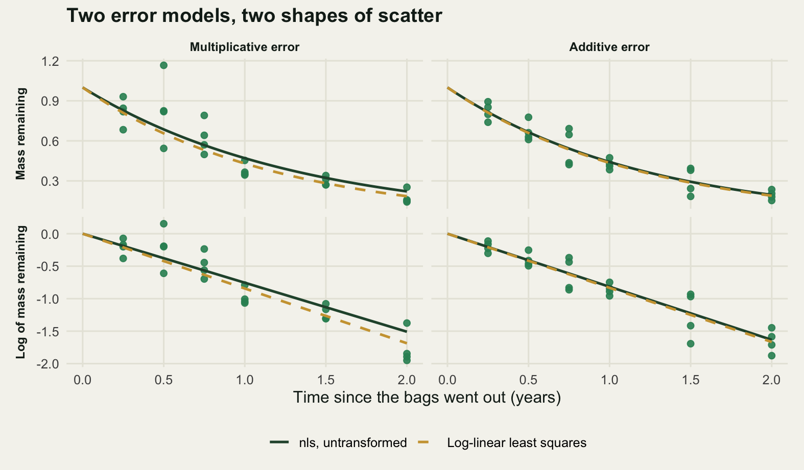
The figure did not do what it was drawn to do, and that is the more useful result. The column where the two curves visibly disagree is the multiplicative one, where the log-linear fit is the estimator built for the job, and the column where they agree is the additive one, where it is not. The gap between the two fits on a single study is noise, and its size carries no information about which of them is right. That only shows up over repeated studies, which is the next section.
What the panels do show is the weighting argument. Ordinary least squares gives every point the same weight, and on the log scale a bag holding a twentieth of its mass is one point like any other. But the log of a small measured mass is a wildly uncertain quantity. An absolute error that moves an early bag from eight tenths to three quarters moves its log a little; the same absolute error at one tenth moves the log a great deal. That is the bottom right panel: additive noise, viewed on the log scale, fans out towards the end of the study. So the log-linear fit does not down-weight the noisy end, it promotes it, and the noisiest points are the ones furthest out in time, which are also the points that pull hardest on a slope. On the arithmetic scale directly above, the same points look reassuringly close to the curve.
What the error model costs
One draw is anecdote. Cross the two estimators against the two generators over a thousand replicates and the pattern is measurable.
n_rep <- 1000
set.seed(20260726)
est <- array(NA_real_, c(n_rep, 2, 2))
n_neg <- 0
for (i in seq_len(n_rep)) {
  ym <- mu * exp(rnorm(length(tv), 0, sig_mult))
  ya <- mu + rnorm(length(tv), 0, sig_add)
  n_neg <- n_neg + sum(ya <= 0)
  est[i, 1, 1] <- k_loglin(ym, tv); est[i, 1, 2] <- k_nls(ym, tv)
  est[i, 2, 1] <- k_loglin(ya, tv); est[i, 2, 2] <- k_nls(ya, tv)
}
k_mean <- apply(est, c(2, 3), mean)
k_sd <- apply(est, c(2, 3), sd)
dimnames(k_mean) <- dimnames(k_sd) <-
  list(c("multiplicative", "additive"), c("log_linear", "nls"))
print(round(k_mean, 4))
log_linear nls
multiplicative 0.7994 0.7833
additive 0.8403 0.8024print(round(k_sd, 4)) log_linear nls
multiplicative 0.0323 0.0439
additive 0.0809 0.0477round(c(replicates = n_rep, true_k = k_true,
bags_simulated = n_rep * length(tv),
bags_at_or_below_zero_under_the_additive_model = n_neg,
loglin_bias_on_additive_percent =
100 * (k_mean["additive", "log_linear"] / k_true - 1),
nls_bias_on_multiplicative_percent =
100 * (k_mean["multiplicative", "nls"] / k_true - 1),
sd_ratio_on_additive_data =
k_sd["additive", "log_linear"] / k_sd["additive", "nls"],
sd_ratio_on_multiplicative_data =
k_sd["multiplicative", "nls"] / k_sd["multiplicative", "log_linear"]), 4) replicates
1000.0000
true_k
0.8000
bags_simulated
24000.0000
bags_at_or_below_zero_under_the_additive_model
69.0000
loglin_bias_on_additive_percent
5.0377
nls_bias_on_multiplicative_percent
-2.0817
sd_ratio_on_additive_data
1.6966
sd_ratio_on_multiplicative_data
1.3598 Read the two-by-two along its diagonal first. Each estimator lands close to the truth when it is matched to the generator that made the data: the log-linear fit returns 0.7994 on multiplicative error and nls returns 0.8024 on additive error, against a true 0.8.
Off the diagonal the two mismatches go in opposite directions. Fed additive error, the log-linear estimator returns 0.8403, too fast by 5.0377 per cent, for the reason the figure showed: it takes the log of noisy small numbers, and the downward pull of a bad late bag is stronger than the upward pull of a good one. Fed multiplicative error, nls returns 0.7833, too slow by 2.0817 per cent, because multiplicative noise lifts the arithmetic mean of the mass remaining above the median curve, and a fit anchored at M0 equal to one can only absorb that by flattening.
The variance matters more than either bias. Under additive error the log-linear estimator has 1.6966 times the standard deviation of nls; under multiplicative error nls has 1.3598 times the standard deviation of the log-linear fit. The wrong error model costs a few per cent of accuracy and a much larger share of the precision, and it is the precision loss that will quietly sink a comparison between two site means.
taylor <- k_true + sig_add^2 / 2 * sum(tv / mu^2) / sum(tv^2)
round(c(log_linear_on_additive_simulated = k_mean["additive", "log_linear"],
        log_linear_on_additive_from_the_expansion = taylor,
        nls_on_multiplicative_simulated = k_mean["multiplicative", "nls"],
        nls_on_multiplicative_fitted_to_the_mean_curve =
          k_nls(mu * exp(sig_mult^2 / 2), tv),
        chance_a_bag_falls_below_zero_at_two_years =
          pnorm(0, exp(-k_true * 2), sig_add),
        chance_at_three_years = pnorm(0, exp(-k_true * 3), sig_add)), 4)
log_linear_on_additive_simulated
0.8403
log_linear_on_additive_from_the_expansion
0.8369
nls_on_multiplicative_simulated
0.7833
nls_on_multiplicative_fitted_to_the_mean_curve
0.7813
chance_a_bag_falls_below_zero_at_two_years
0.0122
chance_at_three_years
0.1559 Both off-diagonal cells have a closed form to check them against, which is the only way to know that the simulator and the argument are the same model. For additive noise of size s about a mean m, a second-order expansion gives the expectation of log(y) as log(m) - s^2 / (2 * m^2), so every point is pulled down and the late points, where m is small, are pulled down hardest. Push that through the slope formula and the expansion predicts 0.8369 against a simulated 0.8403. The agreement is good and not perfect, which is what it should be: at the last harvest the noise is close to half the mean, and a second-order expansion is working at the edge of where it is valid. For multiplicative error, fitting the model to the mean curve exp(-k * t) * exp(sig^2 / 2) gives 0.7813 against a simulated 0.7833.
The last two numbers are a warning about the additive model rather than about the fit. Constant additive variance puts real probability on a bag coming back with less than nothing: 0.0122 at the two-year harvest, and 0.1559 if the same study ran on to three years. Over the thousand replicates, 69 of the 24000 simulated bags did exactly that. Additive constant variance is a workable description of a study that stops while most of the mass is still there, and an incoherent one for a study that runs into the tail. That is a reason to prefer the log scale which has nothing to do with which fit is easier.
lab <- c("Log-linear least squares", "nls, untransformed")
gen <- c("Multiplicative (lognormal) error", "Additive (constant variance) error")
ed <- data.frame(
  estimator = factor(rep(lab, 2), levels = lab),
  gen = factor(rep(gen, each = 2), levels = gen),
  mean = c(k_mean[1, 1], k_mean[1, 2], k_mean[2, 1], k_mean[2, 2]),
  lo = c(quantile(est[, 1, 1], 0.025), quantile(est[, 1, 2], 0.025),
         quantile(est[, 2, 1], 0.025), quantile(est[, 2, 2], 0.025)),
  hi = c(quantile(est[, 1, 1], 0.975), quantile(est[, 1, 2], 0.975),
         quantile(est[, 2, 1], 0.975), quantile(est[, 2, 2], 0.975)))
ed$x <- as.numeric(ed$gen) + ifelse(ed$estimator == lab[1], -0.18, 0.18)

ggplot(ed, aes(x, mean, ymin = lo, ymax = hi, colour = estimator)) +
  geom_hline(yintercept = k_true, linetype = 2, colour = te_pal$ink,
             linewidth = 0.6) +
  annotate("text", x = 1.5, y = k_true, vjust = -0.7, hjust = 0.5, size = 3.2,
           colour = te_pal$ink,
           label = paste("true k =", sprintf("%.2f", k_true))) +
  geom_pointrange(size = 0.7, linewidth = 0.9) +
  geom_text(aes(y = hi, label = sprintf("%.3f", mean)), vjust = -0.8,
            size = 3.2, colour = te_pal$ink, show.legend = FALSE) +
  scale_colour_manual(values = c(te_pal$forest, te_pal$gold), name = NULL) +
  scale_x_continuous(breaks = c(1, 2), labels = gen, limits = c(0.6, 2.4)) +
  scale_y_continuous(limits = c(min(ed$lo) - 0.03, max(ed$hi) + 0.045)) +
  labs(x = NULL, y = "Estimated decay constant k (per year)",
       title = "Each estimator is honest only about its own error model") +
  theme_te() +
  theme(axis.text.x = element_text(colour = te_pal$ink, size = 10),
        plot.margin = margin(6, 14, 6, 6))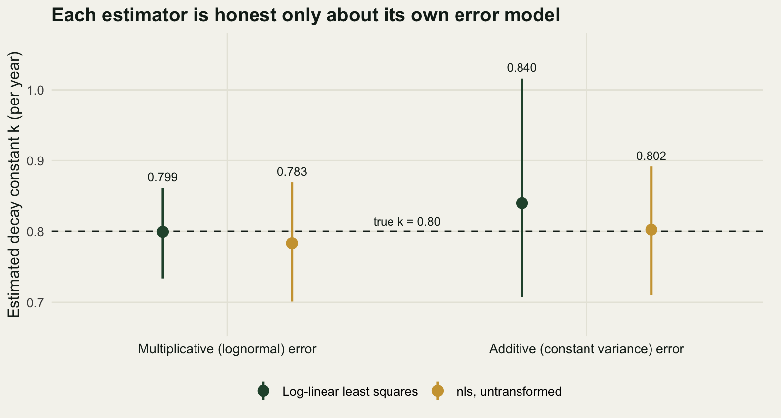
The intercept is not free
Almost every litterbag paper fixes M0 at one. Every bag started at one hundred per cent of itself, so where else would the curve start.
The trouble is what happens between weighing the litter out and the first harvest. Bags shed fragments in transport. Air-dried mass is not oven-dried mass, and the conversion is estimated from a subsample. Some of the finest material falls through the mesh in the first storm, which is loss but not decomposition. Ash contamination pushes the other way. The net result is that the curve the data actually follow starts a little below or above one, and forcing it through one tilts the fitted line to compensate.
The simulation below puts a three per cent handling loss before the first harvest and fits k twice: once with M0 fixed at one, once with the intercept free. Both fits are log-linear on multiplicatively generated data, so the error model is matched and the only thing that changes is the intercept. Two study lengths: a one-year study with four harvests, and a three-year study with five.
handling_loss <- 0.03
M0_true <- 1 - handling_loss
short <- c(0.25, 0.5, 0.75, 1)
long <- c(0.25, 0.5, 1, 2, 3)

intercept_sim <- function(h, n_rep = 6000, seed = 20260726) {
  set.seed(seed)
  t <- rep(h, each = n_bag)
  lmu <- log(M0_true) - k_true * t
  kf <- kr <- m0 <- numeric(n_rep)
  for (i in seq_len(n_rep)) {
    ly <- lmu + rnorm(length(t), 0, sig_mult)
    kf[i] <- -sum(t * ly) / sum(t^2)
    cf <- coef(lm(ly ~ t))
    kr[i] <- -cf[[2]]
    m0[i] <- exp(cf[[1]])
  }
  lev <- sum(t) / sum(t^2)
  c(k_fixed = mean(kf), k_free = mean(kr), M0_estimated = mean(m0),
    sd_fixed = sd(kf), sd_free = sd(kr),
    bias_fixed = mean(kf) - k_true,
    bias_from_the_formula = -log(M0_true) * lev,
    monte_carlo_se = sd(kf) / sqrt(n_rep),
    rmse_fixed = sqrt(mean((kf - k_true)^2)),
    rmse_free = sqrt(mean((kr - k_true)^2)),
    loss_at_which_freeing_M0_pays =
      1 - exp(-sqrt(max(0, var(kr) - var(kf))) / lev))
}
one_year <- intercept_sim(short)
three_year <- intercept_sim(long)
print(round(rbind(one_year_study = one_year, three_year_study = three_year), 4))
k_fixed k_free M0_estimated sd_fixed sd_free bias_fixed
one_year_study 0.8398 0.7975 0.9746 0.0664 0.1600 0.0398
three_year_study 0.8142 0.7997 0.9719 0.0238 0.0394 0.0142
bias_from_the_formula monte_carlo_se rmse_fixed rmse_free
one_year_study 0.0406 9e-04 0.0774 0.1600
three_year_study 0.0144 3e-04 0.0277 0.0394
loss_at_which_freeing_M0_pays
one_year_study 0.1034
three_year_study 0.0644round(c(true_k = k_true, handling_loss = handling_loss, true_M0 = M0_true,
bias_ratio_short_over_long =
one_year[["bias_fixed"]] / three_year[["bias_fixed"]],
percent_bias_one_year = 100 * one_year[["bias_fixed"]] / k_true,
percent_bias_three_year = 100 * three_year[["bias_fixed"]] / k_true,
rmse_ratio_one_year = one_year[["rmse_free"]] / one_year[["rmse_fixed"]],
formula_minus_simulated_percent_of_k =
100 * (one_year[["bias_from_the_formula"]] - one_year[["bias_fixed"]]) / k_true,
monte_carlo_se_percent_of_k = 100 * one_year[["monte_carlo_se"]] / k_true,
crossover_loss_one_year_percent =
100 * one_year[["loss_at_which_freeing_M0_pays"]],
crossover_loss_three_year_percent =
100 * three_year[["loss_at_which_freeing_M0_pays"]]), 4) true_k handling_loss
0.8000 0.0300
true_M0 bias_ratio_short_over_long
0.9700 2.7942
percent_bias_one_year percent_bias_three_year
4.9746 1.7803
rmse_ratio_one_year formula_minus_simulated_percent_of_k
2.0673 0.1020
monte_carlo_se_percent_of_k crossover_loss_one_year_percent
0.1071 10.3423
crossover_loss_three_year_percent
6.4419 Fixing M0 biases k upward, as it must: the fit has to leave the origin at one and arrive at data that are three per cent low, so it leans steeper. In the one-year study the mean estimate is 0.8398, a bias of 4.9746 per cent. In the three-year study it is 0.8142, a bias of 1.7803 per cent. The short study carries 2.7942 times the bias of the long one, and there is nothing mysterious about the ratio. Forcing the line through a point it does not pass through adds -log(M0) * sum(t) / sum(t^2) to the slope, and that term shrinks as the harvests spread out in time. The formula gives 0.0406 for the one-year design against a simulated 0.0398. Those two differ by 0.1020 per cent of k against a Monte Carlo standard error of 0.1071 per cent, so they agree.
Freeing the intercept removes the bias. The free fit returns 0.7975 in the one-year study and recovers M0 at 0.9746 against a true 0.97. That is the textbook answer, and in a short study it is the wrong one.
The measurement contradicted the plan here, so the measurement wins. Freeing M0 in the one-year design costs a great deal of precision, because with four harvest dates crammed into twelve months the intercept and the slope are close to collinear. The standard deviation of k goes from 0.0664 to 0.1600. Put the bias back in and compare root mean squared error: 0.0774 for the fixed fit against 0.1600 for the free one, so on the criterion that counts both kinds of error the free fit is 2.0673 times worse than the fit that is biased on purpose. Freeing the intercept in a one-year study only begins to pay once the handling loss passes 10.3423 per cent, and by three years that crossover has fallen to 6.4419 per cent.
So the rule is not to free the intercept always. It is to free it when the study is long enough for the intercept to be identified from the data, and when it is not, to fix it and report that k is biased upward by an amount you can calculate from the design and a guess at the handling loss.
Study length decides the answer
Everything above assumed the single exponential is true. It is not. Litter is a mixture: sugars, starch and soluble phenolics go in weeks, cellulose in months, lignin and the lignin-bound fraction in years. The simplest description of that is two pools, M(t) = a * exp(-k1 * t) + (1 - a) * exp(-k2 * t), with a labile fraction a decaying at k1 and the rest at a much slower k2.
Now generate from two pools and fit the single exponential, which is what almost every litterbag paper does. There are two simulated litter species: a faster one with a larger labile fraction and a faster slow pool, and a slower one. The study duration is swept from six months to five years, with six harvest dates spread evenly across whatever the duration is and four bags per date, so effort is held constant and only the window changes. The error is multiplicative and the fit is log-linear, so the error model is matched and nothing in this section is contaminated by the previous one.
two_pool <- function(t, a, k1, k2) a * exp(-k1 * t) + (1 - a) * exp(-k2 * t)
sp_a <- c(a = 0.30, k1 = 4.0, k2 = 0.20)
sp_b <- c(a = 0.22, k1 = 4.0, k2 = 0.14)
durations <- c(0.5, 1, 2, 3, 5)
n_harv <- 6

sweep_duration <- function(sp, n_rep = 800, seed = 20260726) {
  set.seed(seed)
  out <- t(sapply(durations, function(dur) {
    h <- dur * seq_len(n_harv) / n_harv
    t <- rep(h, each = n_bag)
    lmu <- log(two_pool(t, sp[["a"]], sp[["k1"]], sp[["k2"]]))
    kf <- kr <- numeric(n_rep)
    for (i in seq_len(n_rep)) {
      ly <- lmu + rnorm(length(t), 0, sig_mult)
      kf[i] <- -sum(t * ly) / sum(t^2)
      kr[i] <- -coef(lm(ly ~ t))[[2]]
    }
    c(k_fixed_M0 = mean(kf), k_free_M0 = mean(kr), sd_of_k_fixed_M0 = sd(kf),
      average_rate = -log(two_pool(dur, sp[["a"]], sp[["k1"]], sp[["k2"]])) / dur,
      mass_left = two_pool(dur, sp[["a"]], sp[["k1"]], sp[["k2"]]))
  }))
  rownames(out) <- paste0(durations, "_years")
  out
}
res_a <- sweep_duration(sp_a)
res_b <- sweep_duration(sp_b)
print(round(res_a, 4))
k_fixed_M0 k_free_M0 sd_of_k_fixed_M0 average_rate mass_left
0.5_years 0.8767 0.6845 0.1128 0.7891 0.6740
1_years 0.6330 0.4198 0.0566 0.5471 0.5786
2_years 0.4396 0.2583 0.0307 0.3782 0.4693
3_years 0.3620 0.2205 0.0188 0.3189 0.3842
5_years 0.2985 0.2046 0.0114 0.2713 0.2575print(round(res_b, 4)) k_fixed_M0 k_free_M0 sd_of_k_fixed_M0 average_rate mass_left
0.5_years 0.6236 0.4726 0.1128 0.5567 0.7570
1_years 0.4439 0.2873 0.0566 0.3825 0.6821
2_years 0.3073 0.1784 0.0307 0.2642 0.5896
3_years 0.2527 0.1536 0.0188 0.2228 0.5125
5_years 0.2086 0.1434 0.0114 0.1897 0.3873ka <- res_a[, "k_fixed_M0"]
kb <- res_b[, "k_fixed_M0"]
round(c(six_month_k_species_a = ka[[1]], five_year_k_species_a = ka[[5]],
ratio_six_months_to_five_years = ka[[1]] / ka[[5]],
species_contrast_at_one_year = ka[[2]] - kb[[2]],
duration_spread_species_a = ka[[1]] - ka[[5]],
spread_over_contrast = (ka[[1]] - ka[[5]]) / (ka[[2]] - kb[[2]]),
one_year_against_three_year_species_a = ka[[2]] - ka[[4]],
species_a_at_two_years = ka[[3]], species_b_at_one_year = kb[[2]],
gap_between_those_two = kb[[2]] - ka[[3]],
sd_of_one_study_species_a_at_two_years = res_a[3, "sd_of_k_fixed_M0"],
slow_pool_rate_species_a = sp_a[["k2"]],
free_M0_fit_at_five_years_species_a = res_a[5, "k_free_M0"],
slow_pool_rate_species_b = sp_b[["k2"]],
free_M0_fit_at_five_years_species_b = res_b[5, "k_free_M0"]), 4) six_month_k_species_a five_year_k_species_a
0.8767 0.2985
ratio_six_months_to_five_years species_contrast_at_one_year
2.9372 0.1891
duration_spread_species_a spread_over_contrast
0.5782 3.0578
one_year_against_three_year_species_a species_a_at_two_years
0.2710 0.4396
species_b_at_one_year gap_between_those_two
0.4439 0.0043
sd_of_one_study_species_a_at_two_years slow_pool_rate_species_a
0.0307 0.2000
free_M0_fit_at_five_years_species_a slow_pool_rate_species_b
0.2046 0.1400
free_M0_fit_at_five_years_species_b
0.1434 sl <- c("Species A, single exponential fit", "Species B, single exponential fit",
"Species A, average instantaneous rate")
dd <- rbind(
data.frame(dur = durations, k = res_a[, "k_fixed_M0"], series = sl[1]),
data.frame(dur = durations, k = res_b[, "k_fixed_M0"], series = sl[2]),
data.frame(dur = durations, k = res_a[, "average_rate"], series = sl[3]))
dd$series <- factor(dd$series, levels = sl)
ggplot(dd, aes(dur, k, colour = series, linetype = series, shape = series)) +
annotate("segment", x = 0.9, xend = 2.55, y = kb[[2]], yend = kb[[2]],
linetype = 3, colour = te_pal$ink, linewidth = 0.6) +
annotate("text", x = 2.65, y = kb[[2]], hjust = 0, size = 3.2,
colour = te_pal$ink, label = "Species B at one year") +
geom_line(linewidth = 0.9) +
geom_point(size = 2.6) +
scale_colour_manual(values = c(te_pal$forest, te_pal$clay, te_pal$gold),
name = NULL) +
scale_linetype_manual(values = c(1, 1, 2), name = NULL) +
scale_shape_manual(values = c(16, 17, 32), name = NULL) +
scale_x_continuous(breaks = durations, limits = c(0.4, 5.4)) +
scale_y_continuous(limits = c(0.15, 0.95)) +
guides(colour = guide_legend(nrow = 2), linetype = guide_legend(nrow = 2),
shape = guide_legend(nrow = 2)) +
labs(x = "Length of the study (years)",
y = "Decay constant k (per year)",
title = "The same litter, a different answer at every duration") +
theme_te() +
theme(plot.margin = margin(6, 14, 6, 6))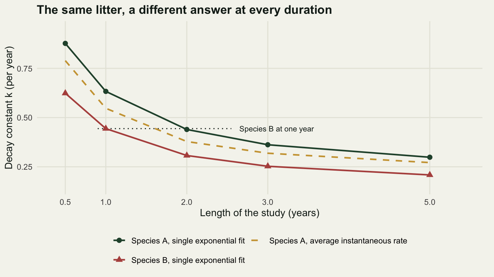
Species A returns 0.8767 per year from a six-month study and 0.2985 per year from a five-year one, a ratio of 2.9372. Nothing about the litter changed. The fit is dominated by whichever phase of the curve the harvests happen to cover, and a short study covers the labile phase almost exclusively. The dashed reference line makes the mechanism concrete: the average instantaneous rate of the true curve over the window falls in the same way, and the single-pool fit tracks it with a small upward offset that comes from forcing M0 to one.
Now put a number on what that does to a comparison. At one year the contrast between the two species is 0.1891 per year, and that contrast is the thing the study was designed to detect. The spread that species A alone shows across the duration sweep is 0.5782 per year, which is 3.0578 times the species contrast. Even the narrower comparison, a one-year study against a three-year study of the same litter, moves k by 0.2710, which is still more than the species difference.
The consequence is worth stating plainly, because it is the reason meta-analyses of k are hard. A two-year study of the faster species A reports 0.4396. A one-year study of the slower species B reports 0.4439. The gap between them is 0.0043, against a standard deviation of 0.0307 for a single study of that size, so no litterbag experiment of that size could tell those two numbers apart. A real difference between two litters has been cancelled exactly by a one-year difference in when somebody stopped collecting.
One more line in the printout is worth reading. Fitting with M0 free instead of fixed gives 0.2046 at five years for species A against a true slow-pool rate of 0.20, and 0.1434 for species B against 0.14. A long study with a free intercept is not estimating an average decay rate at all: it is estimating the slow pool, with the labile pool swallowed into the intercept. That is a different quantity with a different meaning, and which one you end up with depends on a modelling choice made before the data were collected. What the intercept is doing in that fit, and what happens when the curve is allowed an asymptote, is the subject of the recalcitrant pool and the asymptote.
The residual pattern, and whether anyone can see it
A single exponential fitted to two-pool litter has to misfit in a systematic way, and the residuals against time are where it shows. The fit is too shallow in one stretch and too steep in another, and either way the signs of the residuals arrive in runs rather than at random.
Runs are countable, so this does not have to be eyeballed. Order the residuals by harvest date, take their signs, count the runs of like sign, and compare with what independent signs would give. With n1 positive and n2 negative residuals the expected number of runs is 2 * n1 * n2 / (n1 + n2) + 1, and the exact distribution under independence is the Wald-Wolfowitz one, which is a few lines of choose.
runs_count <- function(s) 1 + sum(s[-1] != s[-length(s)])

runs_p <- function(n1, n2, r) {
  n <- n1 + n2
  term <- function(rr) {
    if (rr %% 2 == 0) {
      u <- rr / 2
      2 * choose(n1 - 1, u - 1) * choose(n2 - 1, u - 1) / choose(n, n1)
    } else {
      u <- (rr - 1) / 2
      (choose(n1 - 1, u) * choose(n2 - 1, u - 1) +
         choose(n1 - 1, u - 1) * choose(n2 - 1, u)) / choose(n, n1)
    }
  }
  sum(vapply(2:r, term, numeric(1)))
}

alpha <- 0.05
end_year <- 2
n_total <- 120
h6 <- end_year * seq_len(6) / 6
l6 <- log(two_pool(h6, sp_a[["a"]], sp_a[["k1"]], sp_a[["k2"]]))

r_fixed <- l6 - (sum(h6 * l6) / sum(h6^2)) * h6
r_free <- as.numeric(residuals(lm(l6 ~ h6)))
summarise_runs <- function(r) {
  s <- sign(r)
  n1 <- sum(s > 0); n2 <- sum(s < 0)
  c(runs = runs_count(s), expected_runs = 2 * n1 * n2 / (n1 + n2) + 1,
    exact_p = runs_p(n1, n2, runs_count(s)), largest_residual = max(abs(r)))
}
print(round(rbind(M0_fixed_at_one = summarise_runs(r_fixed),
                  M0_estimated = summarise_runs(r_free)), 4))
runs expected_runs exact_p largest_residual
M0_fixed_at_one 2 3.6667 0.1333 0.1636
M0_estimated 3 4.0000 0.3000 0.0391print(round(c(residual_signs_with_M0_fixed = sign(r_fixed),
standard_error_of_a_harvest_mean = sig_mult / sqrt(n_total / 6),
misfit_in_standard_errors =
max(abs(r_fixed)) / (sig_mult / sqrt(n_total / 6))), 4)) residual_signs_with_M0_fixed1 residual_signs_with_M0_fixed2
-1.0000 -1.0000
residual_signs_with_M0_fixed3 residual_signs_with_M0_fixed4
-1.0000 -1.0000
residual_signs_with_M0_fixed5 residual_signs_with_M0_fixed6
1.0000 1.0000
standard_error_of_a_harvest_mean misfit_in_standard_errors
0.0402 4.0634 smallest_p <- function(n)
min(vapply(seq_len(n - 1), function(n1) runs_p(n1, n - n1, 2), numeric(1)))
n_grid <- c(5, 6, 8, 10, 12, 15, 20)
round(setNames(vapply(n_grid, smallest_p, numeric(1)),
paste0(n_grid, "_dates")), 4) 5_dates 6_dates 8_dates 10_dates 12_dates 15_dates 20_dates
0.2000 0.1000 0.0286 0.0079 0.0022 0.0003 0.0000 Those residuals are the noiseless ones: the exact misfit of a single exponential to the true two-pool curve, with no sampling error in them at all. With M0 fixed at one the signs run negative, negative, negative, negative, positive, positive, which is 2 runs against 3.6667 expected under independence. The largest misfit is 0.1636 on the log scale against a standard error of 0.0402 for a harvest mean of twenty bags, so the pattern sits 4.0634 standard errors deep and is unmistakable to the eye.
The exact one-sided p-value for that perfect, noise-free pattern is 0.1333.
That is the whole problem in one number. It is not the p-value from an unlucky draw, it is the p-value from the cleanest possible version of the signal at six harvest dates. The last line of the printout says why. With five dates the smallest p-value the runs test can produce is 0.2, with six it is 0.1, and it does not drop below 0.05 until eight dates. Below eight harvests the test cannot reject at the conventional level whatever the residuals do, because there are not enough orderings of so few harvests to put enough probability in the tail.
The other row of the table is the same misfit as the fit that estimates M0 sees it. There the largest residual is 0.0391, which is about the standard error of a harvest mean, because a free intercept absorbs most of the labile pool and the curvature left over is tiny. The diagnostic is weakest exactly where the estimator is best behaved.
With noise added, the question becomes how often the test rejects. The sweep below fixes the total effort at one hundred and twenty bags and splits it across a varying number of harvest dates over two years, so more dates means fewer bags per date. The alternative is the two-pool truth. The null for each fit is data generated from the single exponential that fit would estimate, so the false alarm rate is a genuine null and not a second misspecification.
k_null <- -sum(h6 * l6) / sum(h6^2)
cf_null <- coef(lm(l6 ~ h6))

reject_rate <- function(n, lmu_fun, n_rep = 4000) {
  h <- end_year * seq_len(n) / n
  se <- sig_mult / sqrt(n_total / n)
  tab <- outer(0:n, 0:n, Vectorize(function(n1, r)
    if (r < 2 || n1 < 1 || n1 > n - 1) 1 else runs_p(n1, n - n1, r)))
  ym <- matrix(rnorm(n_rep * n, 0, se), n_rep, n) + rep(lmu_fun(h), each = n_rep)
  hb <- mean(h)
  b <- as.vector(ym %*% (h - hb)) / sum((h - hb)^2)
  res_free <- ym - (rowMeans(ym) - b * hb) %o% rep(1, n) - b %o% h
  res_fixed <- ym + (-as.vector(ym %*% h) / sum(h^2)) %o% h
  rate <- function(rr) {
    pos <- rr > 0
    n1 <- rowSums(pos)
    r <- 1 + rowSums(pos[, -1, drop = FALSE] != pos[, -n, drop = FALSE])
    c(reject = mean(tab[cbind(n1 + 1, r + 1)] < alpha), mean_runs = mean(r))
  }
  c(fixed = rate(res_fixed), free = rate(res_free))
}

set.seed(20260726)
alt <- t(sapply(n_grid, reject_rate,
                lmu_fun = function(h)
                  log(two_pool(h, sp_a[["a"]], sp_a[["k1"]], sp_a[["k2"]]))))
nul <- t(sapply(n_grid, function(n) c(
  fixed = reject_rate(n, function(h) -k_null * h)[["fixed.reject"]],
  free = reject_rate(n, function(h) cf_null[[1]] + cf_null[[2]] * h)[["free.reject"]])))

pw <- cbind(dates = n_grid, bags_per_date = n_total / n_grid,
            power_M0_fixed = alt[, "fixed.reject"],
            power_M0_free = alt[, "free.reject"],
            mean_runs_M0_fixed = alt[, "fixed.mean_runs"],
            expected_runs = n_grid / 2 + 1,
            false_alarm_M0_fixed = nul[, "fixed"],
            false_alarm_M0_free = nul[, "free"])
print(round(pw, 4))
dates bags_per_date power_M0_fixed power_M0_free mean_runs_M0_fixed
[1,] 5 24 0.0000 0.0000 2.0190
[2,] 6 20 0.0000 0.0000 2.0735
[3,] 8 15 0.5495 0.0000 2.2240
[4,] 10 12 0.7672 0.1192 2.4845
[5,] 12 10 0.6168 0.0660 2.8560
[6,] 15 8 0.7160 0.0345 3.5113
[7,] 20 6 0.7428 0.0512 4.8475
expected_runs false_alarm_M0_fixed false_alarm_M0_free
[1,] 3.5 0.0000 0.0000
[2,] 4.0 0.0000 0.0000
[3,] 5.0 0.0170 0.0000
[4,] 6.0 0.0328 0.0200
[5,] 7.0 0.0127 0.0092
[6,] 8.5 0.0170 0.0063
[7,] 11.0 0.0177 0.0092fl <- c("M0 fixed at one", "M0 estimated")
pd <- rbind(
data.frame(n = n_grid, p = alt[, "fixed.reject"], fit = fl[1]),
data.frame(n = n_grid, p = alt[, "free.reject"], fit = fl[2]))
pd$fit <- factor(pd$fit, levels = fl)
ggplot(pd, aes(n, p, colour = fit, shape = fit)) +
annotate("rect", xmin = 4.6, xmax = 7.6, ymin = -0.03, ymax = 1.03,
fill = te_pal$sage, alpha = 0.16) +
annotate("text", x = 6.1, y = 0.87, size = 3.6, colour = te_pal$ink,
fontface = "bold", lineheight = 0.95,
label = "No attainable\np-value is this small") +
geom_hline(yintercept = alpha, linetype = 2, colour = te_pal$ink,
linewidth = 0.6) +
geom_line(linewidth = 0.9) +
geom_point(size = 2.6) +
scale_colour_manual(values = c(te_pal$forest, te_pal$clay), name = NULL) +
scale_shape_manual(values = c(16, 17), name = NULL) +
scale_x_continuous(breaks = n_grid) +
scale_y_continuous(limits = c(-0.03, 1.03)) +
labs(x = "Number of harvest dates, total effort fixed",
y = "Probability of rejecting the single pool",
title = "The diagnostic needs more harvests than a study can afford") +
theme_te() +
theme(plot.margin = margin(6, 14, 6, 6))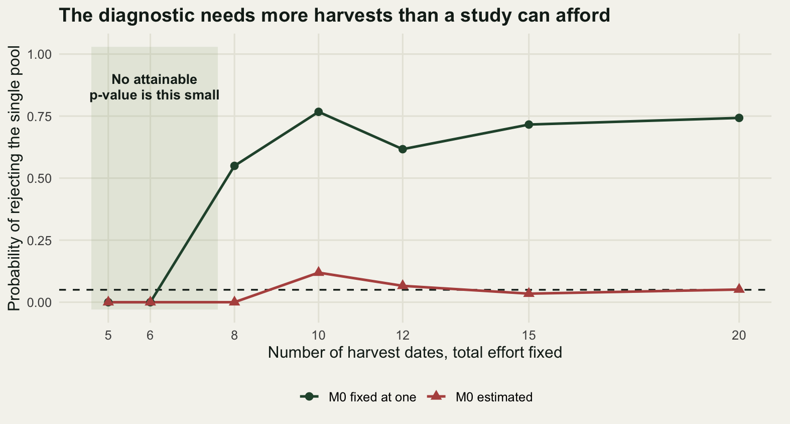
At five and six dates the power is 0, and that zero is exact rather than estimated: no draw of the residuals can produce a p-value under 0.05. The mean number of runs at six dates is 2.0735 against 4.0 expected, so the pattern is there and is being seen; it just cannot be certified. At eight dates the power of the fit with M0 fixed is 0.5495, and at twelve it is 0.6168. The curve is not monotone, and that is not simulation noise: the exact test offers only a handful of attainable significance levels at each number of dates, and the gap between the largest one below 0.05 and the target moves up and down as dates are added.
The fit that estimates M0 is the honest surprise. Its power at twelve dates is 0.0660, barely off its own false alarm rate of 0.0092. The fit that gives the least biased k is also the fit whose residuals carry almost no evidence that the model is wrong, because the free intercept has already absorbed the labile pool. Buying an unbiased estimate costs the ability to find out that the estimate is of the wrong quantity.
The honest limit
Put the sections together and the limit states itself. With five or six harvest dates, which is what a funded litterbag study can afford, the single exponential is not rejected by the data. Not because it is right, and not because the residuals look random: at six dates the noise-free misfit of a two-pool curve sits 4.0634 standard errors deep and still returns a p-value of 0.1333. Choosing the single exponential is therefore a decision and not a result, and it should be reported as one.
Three things follow, and none of them is a statistical fix.
The first is that a k without its study length attached is not interpretable. The same simulated litter gave 0.8767 and 0.2985 here depending only on when the last bag came in. A table of decay constants pooled across studies is a table of two variables added together, and there is no undoing it after the fact, because the duration effect is not a bias with a fixed sign that can be corrected: it depends on the shape of the true curve, which is the thing nobody measured.
The second is that fitting the two-pool model instead does not rescue the situation on its own. Three parameters on six harvest means is a poorly determined problem, the labile rate is anchored by whichever harvests happen to fall in the first few weeks, and the fit can be near-singular in ways that starting values and identifiability sets out in general terms. The companion post the recalcitrant pool and the asymptote takes up what happens when you try.
The third is about this post’s own evidence. Everything here rests on simulated litter whose truth is exactly two exponential pools. Real litter is a continuum of decomposabilities rather than two boxes, and a continuum can produce curves that neither the single exponential nor the two-pool model matches. The measurements above bound how badly the single-pool fit does against a two-pool truth. Against a continuum truth they are a lower bound and not an estimate.
Where to go next
The estimate of k is only half of what a litterbag study is usually asked for. Mass loss is a proxy for carbon loss and the two are not the same quantity, because the carbon concentration of the residue shifts as the labile fraction goes: mass loss and the carbon budget measures the gap. On the diagnostic side, checking a decomposition analysis collects the checks that catch a decomposition fit before it reaches a table, and checking a nonlinear model does the same for nonlinear fits in general.
If the conclusion you took from the error-model section is that the variance structure is worth modelling rather than assuming, that is the right conclusion, and variance structure and heteroscedasticity covers weighting a nonlinear fit properly instead of choosing between two extremes. The log-transform question in its original setting, where the response is unbounded and the small values are not the noisy ones, is in allometry and log-log regression.
References
Olson JS 1963 Ecology 44(2):322-331 (10.2307/1932179)
Wald A, Wolfowitz J 1940 The Annals of Mathematical Statistics 11(2):147-162 (10.1214/aoms/1177731909)
Wieder RK, Lang GE 1982 Ecology 63(6):1636-1642 (10.2307/1940104)
Adair EC, Parton WJ, Del Grosso SJ, Silver WL, Harmon ME, Hall SA, Burke IC, Hart SC 2008 Global Change Biology 14(11):2636-2660 (10.1111/j.1365-2486.2008.01674.x)
Xiao X, White EP, Hooten MB, Durham SL 2011 Ecology 92(10):1887-1894 (10.1890/11-0538.1)
Cornwell WK, Weedon JT 2014 Methods in Ecology and Evolution 5(2):173-182 (10.1111/2041-210X.12138)
Berg B, McClaugherty C 2014 Plant Litter, Third Edition, Springer (ISBN 978-3-642-38820-0)