Allometry and log-log regression in R

Fit an allometric exponent on the log scale, then back-transform without losing biomass: retransformation bias, and which error model your data support.

Body size is the variable that most other ecological quantities hang off. Metabolic rate, home range, clutch size, leaf area, tree biomass: each one tends to follow a power law of the form Y = a * M^b, and the exponent b is usually the quantity of interest. The standard move is to take logs of both sides, which turns the power law into a straight line, and read the exponent off the slope.

That move is sound. What goes wrong is the trip back. If you fit on the log scale and then exponentiate your predictions, you do not get the average biomass you were trying to predict. You get something systematically smaller, and the gap is large enough to matter for a stand-level carbon estimate.

This post builds a small allometric dataset, fits the exponent, measures the size of the back-transformation gap, and fixes it two ways. Then it asks the question that decides whether you should have logged anything at all: where does the error live?

A power law on the log scale

Take a stand of trees. Each one has a stem diameter and an above-ground dry biomass. The biomass grows faster than linearly with diameter, because a wider stem is also a taller stem carrying a broader crown.

set.seed(379)
n_tree <- 240
b_true <- 2.6
a_true <- 0.062
s_true <- 0.32

diam <- exp(rnorm(n_tree, log(28), 0.55))
biomass <- a_true * diam^b_true * exp(rnorm(n_tree, 0, s_true))

fit_log <- lm(log(biomass) ~ log(diam))
b_hat <- unname(coef(fit_log)[2])
a_hat <- unname(exp(coef(fit_log)[1]))
sigma_hat <- summary(fit_log)$sigma
c(exponent = b_hat, coefficient = a_hat, resid_sd = sigma_hat)

   exponent coefficient    resid_sd 
 2.61532908  0.05889828  0.32389291 

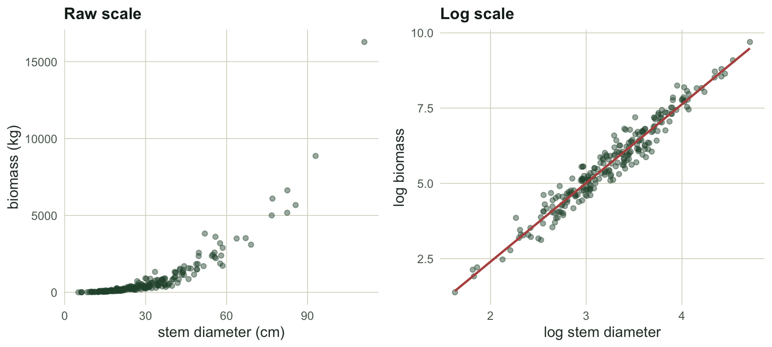
The scatter is generated with a multiplicative error term, exp(rnorm(...)), so a tree is a fixed percentage above or below its expected biomass rather than a fixed number of kilograms. That is the usual situation in biology, and it is exactly what the log transform is built for: on the log scale, a multiplicative error becomes an additive one with constant variance.

The fitted exponent is 2.615 against a true value of 2.60, and the residual standard deviation on the log scale is 0.324.

Figure 1: Tree biomass against stem diameter on the raw scale (left) and after taking natural logs of both variables (right). The power law becomes a straight line, and the scatter becomes even.

The trip back costs you biomass

Now predict. You want each tree’s expected biomass in kilograms, so you exponentiate the fitted values and add them up.

pred_naive <- exp(predict(fit_log))
total_true <- sum(biomass)
total_naive <- sum(pred_naive)
c(true_total = total_true, naive_total = total_naive,
  shortfall_pct = 100 * (total_naive / total_true - 1))

   true_total   naive_total shortfall_pct 
185329.224426 173810.153270     -6.215464 

The predicted stand total falls short of the real one by 6.2 percent. Nothing is wrong with the fit. The gap comes from what exp() does to a symmetric distribution.

On the log scale the residuals sit symmetrically around the fitted line, so the fitted value is the mean of the logs. Exponentiate it and you get the median biomass, not the mean, and for a right-skewed quantity the median sits below the mean. Under lognormal residuals the ratio is exactly exp(-s^2/2), which here is 0.9489.

Two corrections exist, and both are one line.

cf_baskerville <- exp(sigma_hat^2 / 2)
cf_smearing <- mean(exp(residuals(fit_log)))
c(baskerville = cf_baskerville, smearing = cf_smearing,
  baskerville_total = sum(pred_naive) * cf_baskerville,
  smearing_total = sum(pred_naive) * cf_smearing,
  true_total = total_true)

      baskerville          smearing baskerville_total    smearing_total 
     1.053853e+00      1.053967e+00      1.831704e+05      1.831902e+05 
       true_total 
     1.853292e+05 

Baskerville’s factor exp(s^2/2) inverts the lognormal shift analytically. Duan’s smearing estimator does the same job without assuming a distribution: it averages exp(residual) across the sample, letting the observed residuals speak for themselves. Here they give 1.0539 and 1.0540, close enough that the choice does not matter on these data.

One realisation proves nothing, so repeat the whole exercise.

set.seed(3790)
n_rep <- 2000
mc <- t(vapply(seq_len(n_rep), function(i) {
  d <- exp(rnorm(n_tree, log(28), 0.55))
  y <- a_true * d^b_true * exp(rnorm(n_tree, 0, s_true))
  f <- lm(log(y) ~ log(d))
  p <- exp(predict(f))
  s2 <- summary(f)$sigma^2
  c(sum(p) / sum(y),
    sum(p) * exp(s2 / 2) / sum(y),
    sum(p) * mean(exp(residuals(f))) / sum(y))
}, numeric(3)))
mc_mean <- colMeans(mc)
names(mc_mean) <- c("naive", "baskerville", "smearing")
round(c(mc_mean, theory = exp(-s_true^2 / 2)), 4)

      naive baskerville    smearing      theory 
     0.9525      1.0027      1.0023      0.9501 

Across 2,000 simulated stands the naive back-transformation returns 0.9525 of the true total, against the theoretical 0.9501. Both corrections land on 1.003 and 1.002. The shortfall is a bias, not bad luck, and it scales with the residual spread: doubling the log-scale scatter roughly quadruples the exponent in exp(-s^2/2).

Which error model do your data support?

The log transform is not a neutral convenience. Logging the response asserts that the error is multiplicative. Fitting Y = a * M^b directly with nls() asserts that it is additive and of constant size in kilograms. These are different models of the same mean function, and they will not agree.

The tempting question is which one gets the exponent right. Measure it.

set.seed(3793)
n_em <- 1200
em_mult <- t(vapply(seq_len(n_em), function(i) {
  d <- exp(rnorm(n_tree, log(28), 0.55))
  y <- a_true * d^b_true * exp(rnorm(n_tree, 0, 0.32))
  c(unname(coef(lm(log(y) ~ log(d)))[2]),
    tryCatch(unname(coef(nls(y ~ a * d^b, start = list(a = 0.05, b = 2.5)))[2]),
             error = function(e) NA_real_))
}, numeric(2)))
rmse <- function(v) sqrt(mean((v - b_true)^2, na.rm = TRUE))
c(loglog_mean = mean(em_mult[, 1]), nls_mean = mean(em_mult[, 2], na.rm = TRUE),
  loglog_rmse = rmse(em_mult[, 1]), nls_rmse = rmse(em_mult[, 2]),
  rmse_ratio = rmse(em_mult[, 2]) / rmse(em_mult[, 1]))

loglog_mean    nls_mean loglog_rmse    nls_rmse  rmse_ratio 
 2.59927113  2.62031301  0.03899692  0.35157403  9.01543093 

Both estimators are close to the truth on average: 2.599 for the log-log fit and 2.620 for nls(), against 2.60. The cost of picking the wrong error model is not bias. It is spread. The root mean squared error of the nls() exponent is 9.0 times the log-log one, and the middle 95 percent of nls() exponents runs from 2.11 to 3.48 while the log-log fit stays inside 2.53 to 2.68.

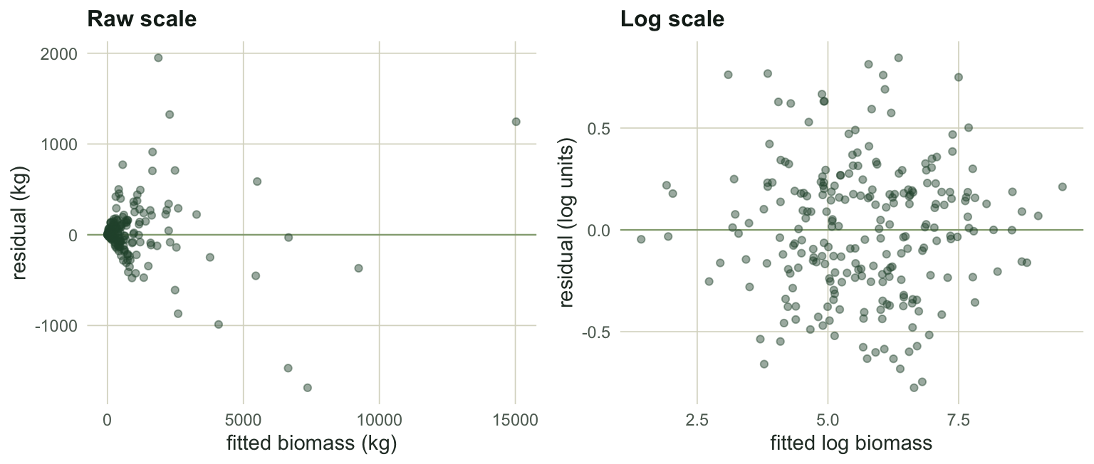
The reason is visible in the data. With multiplicative error, the largest trees carry the largest absolute scatter, so a least-squares fit on the raw scale spends almost all of its attention on a handful of big stems. On the log scale that scatter is even, and every tree contributes.

The comparison runs the other way too. Generate additive, constant-variance error over a narrow diameter range where negative biomass never arises, and nls() becomes the efficient choice.

set.seed(3794)
em_add <- t(vapply(seq_len(n_em), function(i) {
  d <- runif(n_tree, 20, 60)
  mu <- a_true * d^b_true
  y <- mu + rnorm(n_tree, 0, 0.25 * min(mu))
  c(unname(coef(lm(log(y) ~ log(d)))[2]),
    tryCatch(unname(coef(nls(y ~ a * d^b, start = list(a = 0.05, b = 2.5)))[2]),
             error = function(e) NA_real_))
}, numeric(2)))
c(loglog_rmse = rmse(em_add[, 1]), nls_rmse = rmse(em_add[, 2]),
  ratio = rmse(em_add[, 1]) / rmse(em_add[, 2]))

loglog_rmse    nls_rmse       ratio 
 0.03503297  0.01223396  2.86358389 

On additive data the log-log fit has 2.9 times the root mean squared error of nls(). Neither method is better in general. The error distribution decides, and this is the point Xiao and colleagues made after a long argument in the literature about whether log transformation invalidates published power laws.

Figure 2: Residuals from the same multiplicative dataset, plotted on the raw scale (left) and the log scale (right). The raw-scale funnel is the signature of multiplicative error, and it is what the log transform removes.

The residual plot is the diagnostic. A funnel on the raw scale and an even band on the log scale says multiplicative, and the log-log fit is the efficient one. The reverse pattern says additive, and nls() is. If you have never looked, you have chosen by habit.

Where to go next

The workflow for an allometric equation is short: log both variables, fit, check the residual scale, and apply a correction factor before you convert anything back to kilograms. Report the factor you used, because a reader cannot reconstruct it from the coefficients.

Two things this post left open. First, the corrections above assume the log-scale residuals are homoscedastic; if they widen with size, the smearing factor is an average over unlike things and a size-specific correction is needed. Second, and larger, the whole post fitted the slope with ordinary least squares, which assumes the x variable is measured without error. Diameter tape readings are not error free, and body masses even less so. That assumption changes which line you should fit, and it changes the exponent.

Honest limits

Baskerville’s factor is exactly right only under lognormal residuals. The smearing estimator drops that assumption but still needs the residuals to be identically distributed across the size range, and it is noisier in small samples because it averages exp() of a handful of numbers. Neither correction rescues a fit whose functional form is wrong: if the relationship bends on the log scale, no scalar multiplier will repair it.

References

Baskerville 1972 Canadian Journal of Forest Research 2(1):49-53 (10.1139/x72-009)

Duan 1983 Journal of the American Statistical Association 78(383):605-610 (10.1080/01621459.1983.10478017)

Xiao, White, Hooten, Durham 2011 Ecology 92(10):1887-1894 (10.1890/11-0538.1)

Warton, Wright, Falster, Westoby 2006 Biological Reviews 81(2):259-291 (10.1017/S1464793106007007)

Related tutorials

• SMA or OLS for a scaling exponent? - which line to fit when both variables carry error.
• Nonlinear regression with nls - fitting a curve on its own scale instead of linearising it.
• Species-area relationships - another ecological power law, and the log-versus-power choice it forces.
• Checking an allometric analysis - leverage, size range and phylogeny.