Checking an allometric analysis

Three diagnostics for a scaling exponent: where the leverage sits, how much size range separates 2/3 from 3/4, and what shared ancestry does to the test.

The three previous posts built an allometric analysis: log both variables, choose a line, test the exponent. This one asks what could still be wrong with the answer.

The three checks below are not residual plots. They are questions about the design of the sample, and each has a number attached that you can compute before you write anything down: how much of the fit rests on a handful of animals, whether your size range can support the comparison you want to make, and what shared evolutionary history does to a test that assumes independent species.

Check one: where does the leverage sit?

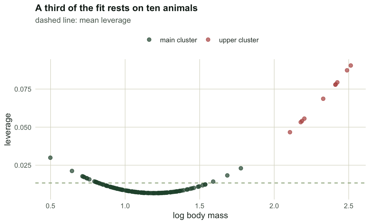
Field allometry datasets have a characteristic shape. Small individuals are easy to catch, weigh and measure, so you get a lot of them. Large ones are rare, slow to process, and sometimes need a different method entirely. The result is many points in a narrow cluster and a few far out on the size axis.

On the log scale, leverage is a function of distance from the mean of x, so those few far points carry the fit.

sma_slope <- function(x, y) sign(cor(x, y)) * sd(y) / sd(x)

set.seed(43826)
n_small <- 140
n_large <- 10
b_true <- 0.75
sd_ex <- 0.16

size_true <- c(rnorm(n_small, log10(12), 0.16), rnorm(n_large, log10(210), 0.10))
log_mass  <- size_true + rnorm(n_small + n_large, 0, sd_ex)
log_trait <- b_true * size_true + rnorm(n_small + n_large, 0, b_true * sd_ex)

hat <- 1 / length(log_mass) +
  (log_mass - mean(log_mass))^2 / sum((log_mass - mean(log_mass))^2)
big <- order(log_mass, decreasing = TRUE)[seq_len(n_large)]
c(pct_of_sample = 100 * n_large / length(log_mass),
  pct_of_leverage = 100 * sum(hat[big]) / sum(hat),
  largest_hat_over_mean = hat[order(log_mass, decreasing = TRUE)[1]] / mean(hat))

        pct_of_sample       pct_of_leverage largest_hat_over_mean 
             6.666667             34.572950              6.785787 

The 6.7 percent of the sample that sits in the upper cluster carries 34.6 percent of the leverage, and the single largest animal has 6.8 times the average. That is not a defect. Spread on the x axis is what makes an exponent estimable, and those animals are earning their place.

The risk is specific: those points have no near neighbours to contradict them. A transcription error on a common small animal is absorbed. The same error on the largest one is not.

biggest  <- order(log_mass, decreasing = TRUE)[1]
smallest <- order(log_mass)[1]
b_base <- sma_slope(log_mass, log_trait)

trait_big_wrong <- log_trait; trait_big_wrong[biggest] <- trait_big_wrong[biggest] + log10(2)
trait_small_wrong <- log_trait; trait_small_wrong[smallest] <- trait_small_wrong[smallest] + log10(2)

c(baseline = b_base,
  largest_doubled = sma_slope(log_mass, trait_big_wrong),
  smallest_doubled = sma_slope(log_mass, trait_small_wrong),
  pct_change_largest = 100 * (sma_slope(log_mass, trait_big_wrong) / b_base - 1),
  pct_change_smallest = 100 * (sma_slope(log_mass, trait_small_wrong) / b_base - 1))

           baseline     largest_doubled    smallest_doubled  pct_change_largest 
          0.7814528           0.7993363           0.7774200           2.2884980 
pct_change_smallest 
         -0.5160628 

One animal recorded at twice its true trait value moves the exponent by +2.3 percent when it is the largest in the sample, and -0.5 percent when it is the smallest. The asymmetry is roughly the leverage ratio, and it is why the practical version of this check is not a statistic at all: go back and re-read the datasheet for your five largest animals.

Figure 1: Leverage against log body mass for a typical field sample. Most of the animals sit in a low-leverage cluster, and a handful at the top of the size range carry a third of the total.

Check two: is your size range wide enough for the question?

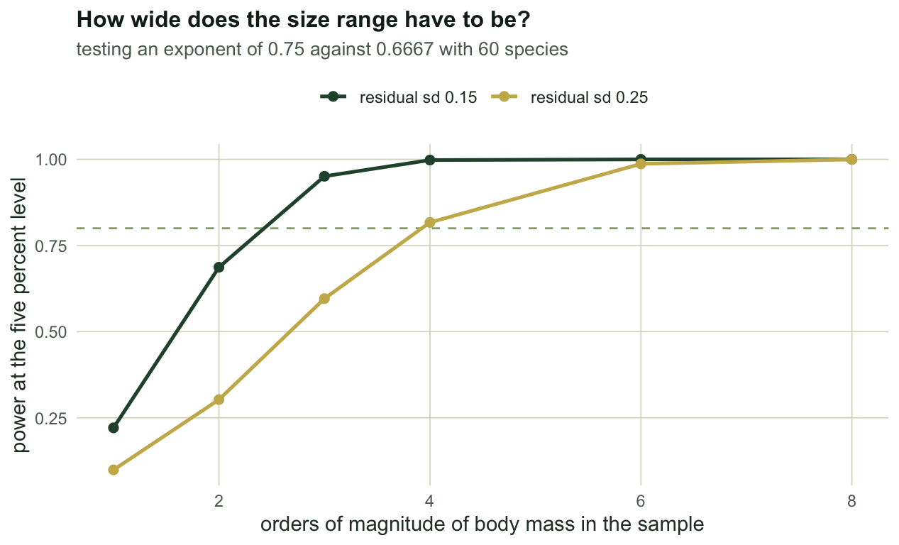
Metabolic scaling has spent decades arguing over whether the exponent is 2/3 or 3/4. Those values differ by 0.0833, which is a small target, and whether your dataset can hit it depends almost entirely on how many orders of magnitude of body mass it covers.

This is a power calculation, and it is worth doing before fieldwork rather than after.

b_alt <- 0.75
b_h0 <- 2 / 3
n_sp <- 60
decades <- c(1, 2, 3, 4, 6, 8)

power_grid <- do.call(rbind, lapply(c(0.15, 0.25), function(sd_res) {
  do.call(rbind, lapply(decades, function(dec) {
    set.seed(4200 + dec + round(sd_res * 100))
    p <- replicate(1500, {
      lx <- runif(n_sp, 0, dec)
      ly <- b_alt * lx + rnorm(n_sp, 0, sd_res)
      co <- summary(lm(ly ~ lx))$coefficients[2, ]
      2 * pt(-abs((co[1] - b_h0) / co[2]), n_sp - 2)
    })
    data.frame(resid_sd = sd_res, orders_of_magnitude = dec,
               power = round(mean(p < 0.05), 3))
  }))
}))
power_grid

   resid_sd orders_of_magnitude power
1      0.15                   1 0.221
2      0.15                   2 0.687
3      0.15                   3 0.951
4      0.15                   4 0.998
5      0.15                   6 1.000
6      0.15                   8 1.000
7      0.25                   1 0.099
8      0.25                   2 0.303
9      0.25                   3 0.596
10     0.25                   4 0.817
11     0.25                   6 0.987
12     0.25                   8 1.000

With 60 species and a residual standard deviation of 0.15 on the log10 scale, a single order of magnitude of body mass gives 22 percent power to distinguish 3/4 from 2/3, and you need 3 orders to clear 80 percent. Loosen the scatter to 0.25, which is not unusual for interspecific data, and one order of magnitude gives 10 percent: the study cannot answer the question it was designed around, and no amount of careful line fitting will change that.

Figure 2: Power to distinguish an exponent of 3/4 from 2/3, as a function of the orders of magnitude of body mass covered and the residual scatter. A narrow size range cannot separate the two hypotheses at any realistic sample size.

Check three: are your species independent?

Interspecific allometry regresses one species trait on another, and the standard tests treat each species as an independent observation. Species are not independent. Two closely related mammals share most of their evolutionary history, so they share most of whatever has pushed their metabolic rate away from the line.

Build a random ultrametric tree, express it as a shared-ancestry covariance matrix, and simulate both traits as Brownian motion on it. Then test a hypothesis that is true.

make_vcv <- function(n_tips) {
  V <- matrix(0, n_tips, n_tips)
  build <- function(idx, height) {
    V[idx, idx] <<- height
    if (length(idx) < 2) return(invisible(NULL))
    deeper <- height + (1 - height) * runif(1, 0.15, 0.6)
    k <- sample.int(length(idx) - 1, 1)
    build(idx[seq_len(k)], deeper)
    build(idx[-seq_len(k)], deeper)
  }
  build(seq_len(n_tips), 0)
  diag(V) <- 1
  V
}

pgls_slope <- function(x, y, V, b0) {
  Vi <- chol2inv(chol(V)); X <- cbind(1, x); n <- length(x)
  bhat <- solve(t(X) %*% Vi %*% X, t(X) %*% Vi %*% y)
  rg <- y - X %*% bhat
  s2 <- as.numeric(t(rg) %*% Vi %*% rg / (n - 2))
  se <- sqrt(s2 * solve(t(X) %*% Vi %*% X)[2, 2])
  c(slope = bhat[2], p = 2 * pt(-abs((bhat[2] - b0) / se), n - 2))
}

The residual in this simulation evolves on the same tree as the trait, which is the situation the phylogenetic comparative literature was built for: the departures from the line are themselves inherited.

n_tips <- 60
b_phy <- 0.75
set.seed(4383)
phy <- t(vapply(seq_len(1200), function(i) {
  V <- make_vcv(n_tips); L <- t(chol(V))
  x <- as.vector(L %*% rnorm(n_tips)) * 1.2
  y <- b_phy * x + as.vector(L %*% rnorm(n_tips)) * 0.35
  co <- summary(lm(y ~ x))$coefficients[2, ]
  p_ols <- 2 * pt(-abs((co[1] - b_phy) / co[2]), n_tips - 2)
  pg <- pgls_slope(x, y, V, b_phy)
  c(p_ols, pg["p"], co[1], pg["slope"])
}, numeric(4)))
c(ols_reject = mean(phy[, 1] < 0.05), pgls_reject = mean(phy[, 2] < 0.05),
  mean_slope_ols = mean(phy[, 3]), mean_slope_pgls = mean(phy[, 4]))

     ols_reject     pgls_reject  mean_slope_ols mean_slope_pgls 
     0.55833333      0.04666667      0.74873782      0.75134431 

The hypothesis is true in every one of these simulated clades. The ordinary least squares test rejects it 55.8 percent of the time; generalised least squares on the phylogenetic covariance holds at 0.047.

Look at the last two numbers before drawing the wrong lesson. The mean least squares slope is 0.7487 and the mean phylogenetic one is 0.7513, both on top of the truth. Ignoring the phylogeny did not bias the exponent. It made the standard error far too small, because the effective number of independent data points is much less than the number of species. The point estimate was fine and the confidence interval was fiction.

What these three checks add up to

A published scaling exponent is a joint product of the line you chose, the size range you sampled, the taxa you happened to include, and the handful of large individuals that anchor the top of the range. The 2/3 against 3/4 argument has run as long as it has partly because those four things vary between studies, and each of them can move an exponent by more than the difference under debate.

The checks are cheap. Compute the leverage distribution and re-read the datasheets for the top few. Run the power grid against the specific alternative you care about, using your own scatter and sample size. If the points are species rather than individuals, put the tree in the model, and quote the interval that comes out rather than the one that does not.

Honest limits

None of this bounds the error from a wrong functional form: every simulation here assumed a genuine power law, and a relationship that bends on the log scale will defeat all three checks. The phylogenetic check assumed Brownian motion on a known tree, and real analyses have neither; a mis-specified branch length model produces its own intervals, correctly calibrated for a process that did not happen. And the power grid is a statement about detecting a difference in the fitted exponent, which is only the biological exponent under the error model the line assumes. These checks constrain the answer. They do not certify it.

References

Warton, Wright, Falster, Westoby 2006 Biological Reviews 81(2):259-291 (10.1017/S1464793106007007)

Felsenstein 1985 The American Naturalist 125(1):1-15 (10.1086/284325)

Xiao, White, Hooten, Durham 2011 Ecology 92(10):1887-1894 (10.1890/11-0538.1)

Related tutorials

• Testing isometry and comparing slopes - the tests these diagnostics are checking.
• SMA or OLS for a scaling exponent? - the line choice that sets the exponent in the first place.
• Phylogenetic generalised least squares - the correction in check three, at full length.
• Allometry and log-log regression in R - the cluster opener.