sma_slope <- function(x, y) sign(cor(x, y)) * sd(y) / sd(x)

pitman_test <- function(x, y, b0) {
  resid_score <- y - b0 * x
  fit_score   <- y + b0 * x
  cor.test(resid_score, fit_score)
}Testing isometry and comparing slopes
R
allometry
body size
hypothesis testing
ecology tutorial
Is the exponent really 3/4? Testing a hypothesised allometric slope, comparing slopes between groups, and separating elevation from a shift along the line.
Corrected 30 September 2026: the elevation test was read as showing no difference; it now says the test found no evidence of a difference. The error sweep said the standardised major axis test settles near nominal once the x error balances the equation error in y; that balance is never reached, and the text now says the rejection rate falls because the slope becomes too noisy to detect the bias. The slope comparison said that differences in measurement precision between groups are the reason to prefer the structural test; it now says they can shift standardised major axis slopes too.
Fitting an exponent is rarely the end of an allometric analysis. The questions that follow are comparisons: is the slope different from the isometric value, is it different from 3/4, do the two sexes scale the same way, does the island population sit above the mainland one. Each of these is a hypothesis about a line, and each has a version that answers the wrong question convincingly.
This post covers three of them. The first is testing a slope against a hypothesised value, where the choice of estimator changes the null rejection rate by an order of magnitude. The second is testing whether several groups share a slope. The third is the distinction that gets lost most often: two groups can sit on the same line and still have very different mean trait values.
Testing a slope against a fixed value
Suppose the true exponent is 0.75 and you want to test that hypothesis. There is a neat exact test that comes straight out of the identity in the previous post. Build two derived variables from the data:
The covariance of those two scores is var(y) - b0^2 * var(x), which is zero exactly when the population standardised major axis slope equals b0. So a plain correlation test on the residual and fitted scores is a test of the slope, and it is exact under bivariate normality rather than asymptotic.
Now the comparison that matters. Simulate data where the null is true, with body size measured imperfectly and the two error variances set so the standardised major axis condition holds, and count how often each approach rejects.
b_null <- 0.75
n_ind <- 60
n_mc <- 3000
sd_ex <- 0.30

set.seed(43811)
res <- t(vapply(seq_len(n_mc), function(i) {
  xt <- rnorm(n_ind, 3, 0.8)
  x <- xt + rnorm(n_ind, 0, sd_ex)
  y <- b_null * xt + rnorm(n_ind, 0, b_null * sd_ex)
  co <- summary(lm(y ~ x))$coefficients[2, ]
  p_ols <- 2 * pt(-abs((co[1] - b_null) / co[2]), n_ind - 2)
  c(p_ols, pitman_test(x, y, b_null)$p.value, co[1], sma_slope(x, y))
}, numeric(4)))
c(ols_reject = mean(res[, 1] < 0.05), pitman_reject = mean(res[, 2] < 0.05),
  mean_ols = mean(res[, 3]), mean_sma = mean(res[, 4]))
ols_reject pitman_reject mean_ols mean_sma
0.48833333 0.04966667 0.65796523 0.75147938 The null is true. The least squares t-test rejects it 48.8 per cent of the time at a nominal five per cent level, and the reason is in the last two numbers: the least squares slope averages 0.658 because measurement error in body size attenuates it, so the test is not testing a false hypothesis, it is testing a true one with a biased estimator. The Pitman test holds at 5.0 per cent.
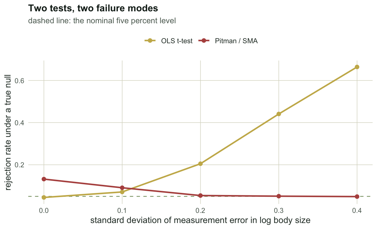
Before concluding that the standardised major axis test is the safe default, sweep the amount of error in x.
sweep_x <- c(0, 0.10, 0.20, 0.30, 0.40)
sw <- do.call(rbind, lapply(seq_along(sweep_x), function(k) {
  su <- sweep_x[k]
  set.seed(9000 + k)
  o <- t(vapply(seq_len(1500), function(i) {
    xt <- rnorm(n_ind, 3, 0.8)
    x <- xt + rnorm(n_ind, 0, su)
    y <- b_null * xt + rnorm(n_ind, 0, sqrt((b_null * su)^2 + 0.12^2))
    co <- summary(lm(y ~ x))$coefficients[2, ]
    c(2 * pt(-abs((co[1] - b_null) / co[2]), n_ind - 2),
      pitman_test(x, y, b_null)$p.value)
  }, numeric(2)))
  data.frame(sd_error_x = su,
             ols = round(mean(o[, 1] < 0.05), 3),
             pitman_sma = round(mean(o[, 2] < 0.05), 3))
}))
sw
sd_error_x ols pitman_sma
1 0.0 0.045 0.132
2 0.1 0.071 0.091
3 0.2 0.205 0.054
4 0.3 0.441 0.051
5 0.4 0.664 0.049Both columns should read 0.05 and neither does everywhere. Least squares climbs from 0.045 to 0.664 as body size gets noisier. The standardised major axis test goes the other way: at 0.132 when x is measured perfectly, then falling to near nominal as the x error grows, but not because the x error comes to balance the equation error in y. That balance is never reached in this sweep: the population standardised major axis slope stays a little above the true exponent throughout, and the extra noise in x only widens the sampling spread of the slope until a sample of this size can no longer detect the bias.
That is the same condition as the previous post, failing here at every level of x error and showing up as a test size rather than as a bias; a larger sample would expose it throughout. There is no estimator here that is safe in both regimes, and the sweep is the honest way to present the choice: you are picking which failure mode you are exposed to.
Elevation is not the same as position along the line
Suppose the common slope test passes and the groups share an exponent. There are still two ways they can differ, and conflating them is the most common error in this corner of the literature.
Construct two groups that lie on exactly the same line, differing only in the body sizes they contain.
set.seed(43822)
b_common <- 0.75
n_grp <- 70
sd_ex2 <- 0.1733
make_group <- function(mean_size) {
  xt <- rnorm(n_grp, mean_size, 0.45)
  list(x = xt + rnorm(n_grp, 0, sd_ex2),
       y = b_common * xt + rnorm(n_grp, 0, b_common * sd_ex2))
}
grp_a <- make_group(2.6)
grp_b <- make_group(3.4)

fit_common <- lr_common(list(grp_a$x, grp_b$x), list(grp_a$y, grp_b$y))
bc <- fit_common$common
res_score <- function(g) g$y - bc * g$x
fit_score <- function(g) g$y + bc * g$x

t_raw <- t.test(grp_a$y, grp_b$y)
t_elev <- t.test(res_score(grp_a), res_score(grp_b))
t_shift <- t.test(fit_score(grp_a), fit_score(grp_b))
c(common_slope = bc, p_raw_means = t_raw$p.value,
  p_elevation = t_elev$p.value, p_shift_along = t_shift$p.value)
common_slope p_raw_means p_elevation p_shift_along
7.335990e-01 1.102082e-12 3.932045e-01 9.470700e-13 The two groups were generated from one relationship with one exponent. The only thing that differs is mean body size.
Compare the raw trait means and you get a p-value of \(1.1 \times 10^{-12}\), which reads as a large and highly significant group difference. Test elevation properly, by comparing residual scores about the common line, and the p-value is 0.393: no evidence of a difference, which is the right verdict, because there is none. Test position along the line and you recover \(9.5 \times 10^{-13}\), which is the real and rather less exciting finding that one group contains larger animals.
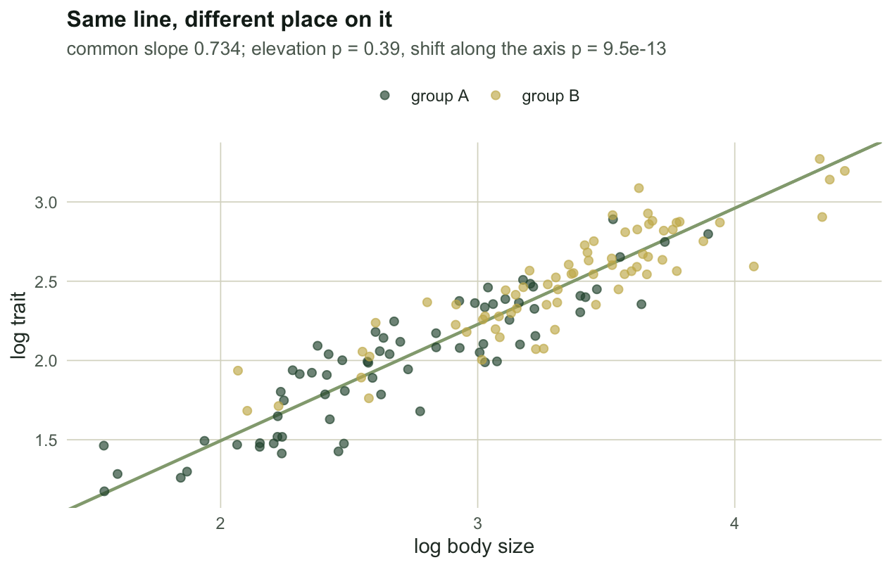
The biological readings are not close. A shift in elevation says that at a given body size, one group has more of the trait: a grade difference, the kind of thing that suggests an adaptive shift. A shift along the axis says only that one group is bigger, and the trait follows along the same rule it always did. Report the second as the first and you have manufactured a result.
Where to go next
The sequence for a grouped allometric comparison runs in a fixed order, because each step depends on the one before. Test for a common slope first; if the slopes differ, elevation is not defined and there is nothing further to compare. If they share a slope, test elevation about the common line. Then, separately, test position along the line, and report it as what it is.
Honest limits
The Pitman test is exact under bivariate normality and only approximate otherwise, and the likelihood ratio test above leans on a chi-squared reference that was checked here for three groups of 45 and no smaller. The whole apparatus tests slopes of the fitted line, which is only the biological exponent under the error model the line assumes. And a common slope test that fails to reject is not evidence that the slopes are equal: with 45 animals per group the power against a difference of 0.17 was 60 per cent, so a null result is compatible with a difference that would matter.
References
Warton, Weber 2002 Biometrical Journal 44(2):161-174 (10.1002/1521-4036(200203)44:2<161::AID-BIMJ161>3.0.CO;2-N)
Warton, Wright, Falster, Westoby 2006 Biological Reviews 81(2):259-291 (10.1017/S1464793106007007)