library(ggplot2)
library(patchwork)

te_paper  <- "#f5f4ee"
te_ink    <- "#16241d"
te_body   <- "#2c3a31"
te_forest <- "#275139"
te_rust   <- "#b5534e"
te_gold   <- "#c9b458"
te_line   <- "#dad9ca"

theme_datasheet <- function() {
  theme_minimal(base_size = 12) +
    theme(plot.background  = element_rect(fill = te_paper, colour = NA),
          panel.background = element_rect(fill = te_paper, colour = NA),
          panel.grid.major = element_line(colour = te_line, linewidth = 0.3),
          panel.grid.minor = element_blank(),
          text             = element_text(colour = te_body),
          plot.title       = element_text(colour = te_ink, face = "bold"),
          plot.subtitle    = element_text(colour = te_body),
          axis.text        = element_text(colour = te_body))
}Ratio indices or ANCOVA for body size
R
ANCOVA
allometry
physiology
simulation
ecology tutorial
Dividing organ mass by body mass invents group effects when fish differ in size. Measuring in R when ratio indices fail, and when ANCOVA fits the wrong curve.
Perch are caught upstream and downstream of a wastewater outfall, thirty from each site, and the liver of every fish is weighed. The liver is the organ that swells when a fish is working hard to clear contaminants, so the question on the sheet is whether the downstream fish have larger livers. The number that goes into the report is the hepatosomatic index: liver mass divided by body mass, times one hundred. It takes one line of R, it has a name, and a two sample t-test on it looks like a direct answer. The downstream fish also happen to be heavier, because the outfall warms the water and the food supply there is better.
Dividing by body mass is a claim about the shape of the relationship. It says that liver mass is proportional to body mass, which is a straight line through the origin. If the real line crosses the liver axis anywhere other than zero, the index changes with body size on its own, and two sites that differ only in the size of their fish will differ in their index. Packard and Boardman 1988 made this argument against ratios in ecophysiology, and Kronmal 1993 made it for ratio standards in general; the remedy both give is to put body size in the model as a covariate, which is the analysis of covariance.
Two posts on this site sit next to the problem without covering it. The post on residuals as a variable deals with condition indices built from a regression: its section on a first stage fitted to somebody else’s data measures what happens when a log-scale index uses a borrowed exponent. That is a residual index, not a raw ratio with a non-zero intercept. The post on testing isometry and comparing slopes separates elevation from position along a shared line, which is exactly the distinction a ratio blurs, but it compares slopes and residual scores rather than testing the ratio itself as a response. And closure and spurious correlation is about the correlations that division by a total invents in compositions, which is the spurious correlation of ratios in a different form, with no group comparison. This post takes the ratio as the response of a group test and measures three things: how often it finds an effect that is not there, what ANCOVA does when its line has the wrong shape and the sites differ in size, and how a real effect can come out of the ratio with the wrong sign.
A ratio is a regression line through the origin
The truth is a straight line with a positive intercept: liver mass is the intercept plus a fixed number of grams per gram of body. Body mass is log-normal inside a site, and the downstream site has its median raised by a given percentage. The scatter around the line is either multiplicative (a constant coefficient of variation, the error model a log-log analysis assumes) or additive (a constant standard deviation). The size of the intercept is set as a share of the mean upstream liver mass, because that share, not the intercept in grams, is what decides how badly the ratio behaves. Every constant below was fixed before any rate was computed.
b_liver  <- 0.012      # grams of liver per gram of body above the intercept
mu_log   <- log(60)    # log median body mass of the upstream fish, grams
sd_log   <- 0.15       # spread of log body mass inside a site
cv_err   <- 0.10       # residual scatter, as a coefficient of variation
n_site   <- 30         # fish per site
alpha_lev <- 0.05
n_rep    <- 4000       # replicate datasets per setting, fixed before any rate was seen
mean_mass <- exp(mu_log + sd_log^2 / 2)

# intercept that makes it a given share of the upstream mean liver mass
icept_for <- function(share) share / (1 - share) * b_liver * mean_mass

draw_sites <- function(n_rep, share, gap, err = "mult", effect = 0, n = n_site,
                       curve = "linear", sdl = sd_log) {
  a  <- icept_for(share)
  x1 <- matrix(rlnorm(n_rep * n, mu_log, sdl), n_rep)
  x2 <- matrix(rlnorm(n_rep * n, mu_log + log(1 + gap), sdl), n_rep)
  if (curve == "linear") {
    f <- function(x) a + b_liver * x
  } else {                                   # power law, exponent 0.75, no intercept
    c_pow <- icept_for(0.3) / 0.3 / mean_mass^0.75
    f <- function(x) c_pow * x^0.75
  }
  m1 <- f(x1); m2 <- f(x2) * (1 + effect)
  if (err == "mult") {
    y1 <- m1 * exp(rnorm(n_rep * n, 0, cv_err))
    y2 <- m2 * exp(rnorm(n_rep * n, 0, cv_err))
  } else {
    sd_add <- cv_err * f(mean_mass)
    y1 <- m1 + rnorm(n_rep * n, 0, sd_add)
    y2 <- m2 + rnorm(n_rep * n, 0, sd_add)
  }
  list(x1 = x1, x2 = x2, y1 = y1, y2 = y2)
}
One dataset first, with the intercept at 30 per cent of the upstream mean liver mass, the downstream fish 30 per cent heavier and no site effect at all. The same data go through the t-test on the index, an ANCOVA of liver mass on body mass and site, and the same ANCOVA on the log scale.
set.seed(3017)
one <- draw_sites(1, share = 0.3, gap = 0.3)
fish <- data.frame(mass  = c(one$x1, one$x2), liver = c(one$y1, one$y2),
                   site  = factor(rep(c("upstream", "downstream"), each = n_site),
                                  levels = c("upstream", "downstream")))
fish$hsi <- 100 * fish$liver / fish$mass
t_hsi  <- t.test(hsi ~ site, data = fish, var.equal = TRUE)
fit_raw <- lm(liver ~ mass + site, data = fish)
fit_log <- lm(log(liver) ~ log(mass) + site, data = fish)
hsi_up <- mean(fish$hsi[fish$site == "upstream"])
hsi_dn <- mean(fish$hsi[fish$site == "downstream"])
p_hsi <- t_hsi$p.value
p_raw <- summary(fit_raw)$coefficients["sitedownstream", 4]
p_log <- summary(fit_log)$coefficients["sitedownstream", 4]
mass_up <- mean(fish$mass[fish$site == "upstream"])
mass_dn <- mean(fish$mass[fish$site == "downstream"])
c(hsi_up = hsi_up, hsi_dn = hsi_dn, p_hsi = p_hsi, p_raw = p_raw, p_log = p_log)
hsi_up hsi_dn p_hsi p_raw p_log
1.750846712 1.604246426 0.003818628 0.354117827 0.459323380 The upstream fish average 59.7 g and the downstream fish 78.1 g. The mean index is 1.75 upstream and 1.60 downstream, and the t-test gives p = 0.0038: a significant result saying the fish below the outfall have relatively smaller livers. The ANCOVA on the raw scale gives p = 0.35 for the site term, and on the log scale p = 0.46. Both are correct, because the two sites were generated from the same line.
The left panel shows where the index result comes from. A fish’s index is the slope of the line from the origin to its point, and each dashed line has the slope of one site’s mean ratio. With a positive intercept, that slope is b + a/X, which falls as body mass rises even for a fish sitting exactly on the true line. The heavier site therefore gets the flatter dashed line and the smaller index, with no difference in liver mass at any given body size.
a_true <- icept_for(0.3)
p_scatter <- ggplot(fish, aes(mass, liver, colour = site)) +
  geom_abline(intercept = a_true, slope = b_liver, colour = te_ink, linewidth = 0.8) +
  geom_abline(intercept = 0, slope = hsi_up / 100, colour = te_forest,
              linetype = "dashed", linewidth = 0.6) +
  geom_abline(intercept = 0, slope = hsi_dn / 100, colour = te_gold,
              linetype = "dashed", linewidth = 0.6) +
  geom_point(size = 2, alpha = 0.8) +
  scale_colour_manual(values = c(te_forest, te_gold), name = NULL) +
  expand_limits(x = 0, y = 0) +
  labs(x = "body mass (g)", y = "liver mass (g)", title = "One line, two ratios",
       subtitle = "solid: true line; dashed: site mean ratio") +
  theme_datasheet() + theme(legend.position = "bottom")
p_index <- ggplot(fish, aes(site, hsi, colour = site)) +
  geom_jitter(width = 0.15, height = 0, size = 1.8, alpha = 0.8, show.legend = FALSE) +
  stat_summary(fun = mean, geom = "crossbar", width = 0.5, colour = te_ink, linewidth = 0.4) +
  scale_colour_manual(values = c(te_forest, te_gold)) +
  labs(x = NULL, y = "liver mass as per cent of body mass", title = "The index",
       subtitle = "bars: site means") +
  theme_datasheet()
p_scatter + p_index + plot_layout(widths = c(2, 1)) +
  plot_annotation(theme = theme_datasheet())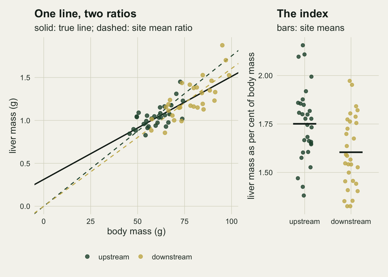
The spurious effect has a formula
Measuring rates needs thousands of datasets per setting, and four fits per dataset. The t-test and the ANCOVA with a common slope both have closed form estimates from sums of squares, so they can be computed for a whole matrix of replicates at once. The ANCOVA site coefficient is the difference in mean response minus the pooled within-site slope times the difference in mean size, and its variance carries the extra term for that difference. A check against t.test and lm on the worked dataset comes first.
pooled_t <- function(a1, a2) {
  m1 <- rowMeans(a1); m2 <- rowMeans(a2)
  v <- (rowSums((a1 - m1)^2) + rowSums((a2 - m2)^2)) / (ncol(a1) + ncol(a2) - 2)
  (m2 - m1) / sqrt(v * (1 / ncol(a1) + 1 / ncol(a2)))
}
ancova_t <- function(xa, xb, ya, yb) {
  mxa <- rowMeans(xa); mxb <- rowMeans(xb); mya <- rowMeans(ya); myb <- rowMeans(yb)
  sxx <- rowSums((xa - mxa)^2) + rowSums((xb - mxb)^2)
  sxy <- rowSums((xa - mxa) * (ya - mya)) + rowSums((xb - mxb) * (yb - myb))
  syy <- rowSums((ya - mya)^2) + rowSums((yb - myb)^2)
  s2 <- (syy - sxy^2 / sxx) / (ncol(xa) + ncol(xb) - 3)
  est <- (myb - mya) - sxy / sxx * (mxb - mxa)
  est / sqrt(s2 * (1 / ncol(xa) + 1 / ncol(xb) + (mxb - mxa)^2 / sxx))
}
four_tests <- function(d) {
  cbind(ratio     = pooled_t(d$y1 / d$x1, d$y2 / d$x2),
        log_ratio = pooled_t(log(d$y1 / d$x1), log(d$y2 / d$x2)),
        ancova    = ancova_t(d$x1, d$x2, d$y1, d$y2),
        log_log   = ancova_t(log(d$x1), log(d$x2), log(d$y1), log(d$y2)))
}
worked_t <- four_tests(one)
lm_t <- c(t_hsi$statistic, summary(fit_raw)$coefficients["sitedownstream", 3],
          summary(fit_log)$coefficients["sitedownstream", 3])
id_gap <- max(abs(abs(worked_t[1, c(1, 3, 4)]) - abs(lm_t)))
The largest difference between the vectorised statistics and the lm and t.test values is 9.8e-15, which is rounding.
The ratio test also has a prediction that needs no simulation. With Y = a + bX times an error of mean k (k = 1 for additive scatter, exp(sigma^2/2) for the log-normal scatter used here), the expected ratio is E[Y/X] = k(b + a E[1/X]). The first term is the same at both sites; the second is not, because heavier fish have a smaller E[1/X]. For log-normal body mass E[1/X] and E[1/X^2] are closed form, so the mean and variance of the ratio at each site are too, and the t statistic has approximately a noncentral t distribution with the standardised difference as its noncentrality. The function below computes that rejection rate for both error models, and the simulation runs over the same grid of intercept shares and size gaps with 4000 datasets per cell.
ratio_power <- function(share, gap, err, n = n_site, alpha = alpha_lev) {
  a <- icept_for(share)
  moments <- function(mu) {
    e1 <- exp(-mu + sd_log^2 / 2); e2 <- exp(-2 * mu + 2 * sd_log^2)  # E[1/X], E[1/X^2]
    if (err == "mult") {
      m  <- (b_liver + a * e1) * exp(cv_err^2 / 2)
      v  <- (b_liver^2 + 2 * a * b_liver * e1 + a^2 * e2) * exp(2 * cv_err^2) - m^2
    } else {
      sd_add <- cv_err * (a + b_liver * mean_mass)
      m <- b_liver + a * e1
      v <- a^2 * (e2 - e1^2) + sd_add^2 * e2
    }
    c(m, v)
  }
  g1 <- moments(mu_log); g2 <- moments(mu_log + log(1 + gap))
  ncp <- (g2[1] - g1[1]) / sqrt((g1[2] + g2[2]) / 2 * 2 / n)
  dfr <- 2 * n - 2; crit <- qt(1 - alpha / 2, dfr)
  pt(-crit, dfr, ncp) + pt(crit, dfr, ncp, lower.tail = FALSE)
}

share_set <- c(0, 0.1, 0.2, 0.3)
gap_set   <- c(0, 0.05, 0.1, 0.15, 0.2, 0.3)
test_lev  <- c("ratio", "log ratio", "ANCOVA", "log-log ANCOVA")
crit2 <- qt(1 - alpha_lev / 2, 2 * n_site - 2)
crit3 <- qt(1 - alpha_lev / 2, 2 * n_site - 3)
set.seed(5521)
grid_tab <- do.call(rbind, lapply(c("mult", "add"), function(err)
  do.call(rbind, lapply(share_set, function(sh)
    do.call(rbind, lapply(gap_set, function(gp) {
      ts <- four_tests(draw_sites(n_rep, sh, gp, err))
      data.frame(err = err, share = sh, gap = gp, test = test_lev,
                 rate = c(mean(abs(ts[, 1]) > crit2), mean(abs(ts[, 2]) > crit2),
                          mean(abs(ts[, 3]) > crit3), mean(abs(ts[, 4]) > crit3)),
                 predicted = c(ratio_power(sh, gp, err), NA, NA, NA))
    }))))))
grid_tab$mcse <- sqrt(grid_tab$rate * (1 - grid_tab$rate) / n_rep)
rt <- function(err, sh, gp, k) grid_tab$rate[grid_tab$err == err & grid_tab$share == sh &
                                              grid_tab$gap == gp & grid_tab$test == test_lev[k]]
pr <- function(err, sh, gp) ratio_power(sh, gp, err)
ratio_rows <- grid_tab[grid_tab$test == "ratio", ]
pred_gap_max <- max(abs(ratio_rows$rate - ratio_rows$predicted))
z_max <- max(abs(ratio_rows$rate - ratio_rows$predicted) / sqrt(ratio_rows$predicted *
                (1 - ratio_rows$predicted) / n_rep))
anc_rows <- grid_tab[grid_tab$test %in% test_lev[3:4], ]
anc_lo <- min(anc_rows$rate); anc_hi <- max(anc_rows$rate)
mcse_05 <- sqrt(alpha_lev * (1 - alpha_lev) / n_rep)
lr_gap <- max(abs(grid_tab$rate[grid_tab$test == "log ratio"] - ratio_rows$rate))
Across the 48 cells of the grid the simulated ratio rate and the noncentral t prediction differ by at most 0.015. In units of the Monte Carlo standard error the largest gap is 2.3, about what the largest of that many standard normal deviates should be, so the prediction holds and the approximation of the ratio by a normal variate costs nothing visible here.
With the intercept at zero the ratio is fine: its rate stays between 0.044 and 0.057 at every size gap. At an intercept of 10 per cent of the mean and a 15 per cent size gap, with multiplicative scatter, the ratio test rejects 7.6 per cent of null experiments (predicted 8.0). At 30 per cent of the mean the same size gap gives 30.0 per cent, and a 30 per cent size gap gives 72.8 per cent. The claim that a modest size difference makes the ratio test fire in most experiments is true only in the top corner of this grid, the largest intercept with the largest gap; at a small intercept it is a moderate inflation, not a certainty.
curve_tab <- expand.grid(share = share_set, gap = seq(0, 0.3, by = 0.005))
curve_tab$predicted <- mapply(ratio_power, curve_tab$share, curve_tab$gap, "mult")
share_lab <- function(s) factor(sprintf("intercept %.0f%% of mean", 100 * s),
                                 levels = sprintf("intercept %.0f%% of mean", 100 * share_set))
curve_tab$share_f <- share_lab(curve_tab$share)
pts <- grid_tab[grid_tab$err == "mult" & grid_tab$test == "ratio", ]
pts$share_f <- share_lab(pts$share)
anc_pts <- grid_tab[grid_tab$err == "mult" & grid_tab$test == "log-log ANCOVA", ]
anc_pts$share_f <- share_lab(anc_pts$share)
ggplot(curve_tab, aes(100 * gap, predicted, colour = share_f)) +
  geom_hline(yintercept = alpha_lev, colour = te_body, linetype = "dashed", linewidth = 0.5) +
  geom_line(linewidth = 0.9) +
  geom_point(data = pts, aes(y = rate), shape = 21, fill = te_paper, size = 2.4, stroke = 0.9) +
  geom_point(data = anc_pts, aes(y = rate), shape = 4, size = 2.2, colour = te_ink,
             show.legend = FALSE) +
  scale_colour_manual(values = c(te_body, te_gold, te_forest, te_rust), name = NULL) +
  scale_y_continuous(limits = c(0, 1)) +
  guides(colour = guide_legend(nrow = 2)) +
  labs(x = "downstream fish heavier by (per cent)", y = "rejection rate, no site effect",
       title = "The ratio test finds a site effect that is not there",
       subtitle = "lines: noncentral t prediction; circles: ratio t-test; crosses: log-log ANCOVA") +
  theme_datasheet() + theme(legend.position = "bottom")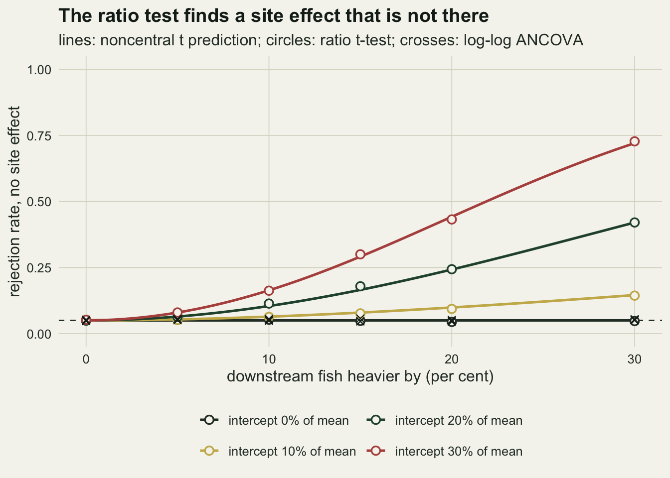
Both ANCOVAs stay between 0.042 and 0.058 over every cell and both error models, against a Monte Carlo standard error of 0.0034 at the nominal level. Switching from multiplicative to additive scatter moves the ratio test a little (at the top corner, 77.5 per cent against 72.8), and the prediction follows it because the variance of the ratio is different under each. Taking logs of the ratio does not help: log(Y/X) is log Y minus log X, which assumes a log-log slope of exactly one, and its rate never differs from the plain ratio’s by more than 0.025.
So far this is arithmetic, and the formula would have given the whole figure. What the formula does not give is how the replacement behaves when the conditions that make it easy are taken away.
When the ANCOVA line has the wrong shape
ANCOVA compares the sites at a common body size by sliding each site along a fitted line to the same mass. If the line has the wrong shape, that slide is wrong by an amount that depends on how far it has to go, which is the difference in mean size between the sites. The usual warning attached to ANCOVA is about overlap: when the sites share no body sizes, the comparison is an extrapolation. Garcia-Berthou 2001 made the case for ANCOVA over residual indices in ecology. This section asks whether overlap or shape is what decides the result.
The test widens the size gap under two truths: the linear line with an intercept used so far, which the raw ANCOVA fits exactly and the log-log ANCOVA does not, and a power law with exponent 0.75 and no intercept, which the log-log ANCOVA fits exactly and the raw ANCOVA does not. The power law is scaled to the same mean liver mass. Overlap is measured as the share of downstream fish lighter than the heaviest upstream fish in the same dataset. Neither truth nor the exponent was chosen after looking at a rate. With the narrow size spread used so far, a large gap and a lack of overlap come together, so a second arm repeats the power law with a wider spread of body mass inside each site; that arm was added after the first results, to pull the two apart, and its one spread value was the only one run.
gap_wide <- c(0, 0.25, 0.5, 0.75, 1, 1.5)
curve_lev <- c("linear with intercept", "power law, exponent 0.75")
err_lev <- c("multiplicative scatter", "additive scatter")
set.seed(7730)
ext_tab <- do.call(rbind, lapply(c("linear", "power"), function(cv)
  do.call(rbind, lapply(c("mult", "add"), function(err)
    do.call(rbind, lapply(gap_wide, function(gp) {
      d <- draw_sites(n_rep, 0.3, gp, err, curve = cv)
      ts <- four_tests(d)
      data.frame(curve = curve_lev[match(cv, c("linear", "power"))],
                 err = err_lev[match(err, c("mult", "add"))], gap = gp,
                 overlap = mean(d$x2 < apply(d$x1, 1, max)),
                 test = test_lev[3:4],
                 rate = c(mean(abs(ts[, 3]) > crit3), mean(abs(ts[, 4]) > crit3)),
                 ratio = mean(abs(ts[, 1]) > crit2))
    }))))))
ext_tab$mcse <- sqrt(ext_tab$rate * (1 - ext_tab$rate) / n_rep)
er <- function(cv, err, gp, k) ext_tab$rate[ext_tab$curve == curve_lev[cv] &
        ext_tab$err == err_lev[err] & ext_tab$gap == gp & ext_tab$test == test_lev[k]]
ov_at <- function(gp) mean(ext_tab$overlap[ext_tab$gap == gp])
ratio_min_wide <- min(ext_tab$ratio[ext_tab$gap >= 1])
loglog_max <- max(ext_tab$rate[ext_tab$test == "log-log ANCOVA"])

# larger sample, the same no-overlap design
n_big <- 120; n_rep_big <- 2000
set.seed(7731)
big <- do.call(rbind, lapply(c("linear", "power"), function(cv)
  do.call(rbind, lapply(c("mult", "add"), function(err) {
    ts <- four_tests(draw_sites(n_rep_big, 0.3, 1, err, n = n_big, curve = cv))
    cr <- qt(1 - alpha_lev / 2, 2 * n_big - 3)
    data.frame(curve = cv, err = err, ancova = mean(abs(ts[, 3]) > cr),
               log_log = mean(abs(ts[, 4]) > cr))
  }))))
bg <- function(cv, err, col) big[big$curve == cv & big$err == err, col]
mcse_big <- sqrt(alpha_lev * (1 - alpha_lev) / n_rep_big)

# the power law again, with a wider size spread so the ranges keep overlapping
sd_wide <- 0.5
set.seed(7733)
wide_tab <- do.call(rbind, lapply(c("mult", "add"), function(err)
  do.call(rbind, lapply(gap_wide, function(gp) {
    d <- draw_sites(n_rep, 0.3, gp, err, curve = "power", sdl = sd_wide)
    data.frame(curve = curve_lev[2], err = err_lev[match(err, c("mult", "add"))], gap = gp,
               overlap = mean(d$x2 < apply(d$x1, 1, max)),
               neg = sum(c(d$y1, d$y2) <= 0),
               rate = mean(abs(ancova_t(d$x1, d$x2, d$y1, d$y2)) > crit3))
  }))))
wide_tab$mcse <- sqrt(wide_tab$rate * (1 - wide_tab$rate) / n_rep)
wr <- function(err, gp, col = "rate") wide_tab[wide_tab$err == err_lev[err] & wide_tab$gap == gp, col]
set.seed(7735)
wide_big <- sapply(c("mult", "add"), function(err) {
  d <- draw_sites(n_rep_big, 0.3, 1, err, n = n_big, curve = "power", sdl = sd_wide)
  c(overlap = mean(d$x2 < apply(d$x1, 1, max)),
    rate = mean(abs(ancova_t(d$x1, d$x2, d$y1, d$y2)) > qt(1 - alpha_lev / 2, 2 * n_big - 3)))
})
At no size gap the overlap measure is 0.97; at a 50 per cent gap it is 0.28 and at a doubling of median mass 0.011, so by then the two sites share almost no body sizes. At a doubling of mass or more the ratio test rejects essentially every null dataset (the lowest rate over those cells is 100.0 per cent), under both truths, including the power law with no intercept at all: a log-log slope below one breaks the ratio just as an intercept does.
The ANCOVAs behave very differently from each other. The log-log ANCOVA never rises above 0.055 anywhere in the grid, including on the linear truth it does not fit. The raw ANCOVA holds on its own truth with additive scatter (0.048 at a gap of 150 per cent), creeps up with multiplicative scatter (0.089), and fails on the power law, reaching 0.123 with multiplicative and 0.125 with additive scatter at the widest gap. The contrast between the two linear panels points to a variance problem for the first rise: multiplicative scatter makes the heavier site noisier, and the pooled residual variance of the raw ANCOVA ignores that. The second rise, on the power law, is the subject of the rest of this section.
Lack of overlap is not what drives it. With the standard deviation of log body mass raised from 0.15 to 0.50, 72 per cent of downstream fish still lie inside the upstream range at a doubling of mass, and the raw ANCOVA rejects 0.138 (multiplicative) and 0.221 (additive) of null datasets there, more than the 0.093 and 0.071 of the narrow spread where the ranges had separated. At a 150 per cent gap, with 57 per cent overlap, the rates are 0.282 and 0.507. The additive arm at this spread can give a small fish a negative liver mass (it happened to at most 1 of the 240000 simulated livers in any cell), which the raw ANCOVA does not notice and a log analysis cannot take, so the wider-spread arm runs only the raw ANCOVA, under both error models. The bias in the site term grows with the difference in mean size whether or not the ranges overlap: a straight line fitted to a curve is the wrong model at every gap, and non-overlap only removes the fish that would have shown the bend.
A bias from the wrong shape does not shrink with sample size, but the standard error of the site term does. With 120 fish per site and a doubling of mass, the raw ANCOVA rejects 0.138 and 0.155 of null datasets on the power law with the narrow spread, against 0.093 and 0.071 with 30, and 0.451 and 0.732 with the wide spread, where 86 per cent of downstream fish overlap. The log-log ANCOVA on the linear truth gives 0.058 and 0.042 (Monte Carlo standard error near the nominal level 0.0049).
That asymmetry is not a difference in curvature. The two wrong fits face curves that bend about equally over a doubling of mass, and the difference is in how the common slope is built. The pooled within-site slope is a weighted mean of the two sites’ own slopes, each weighted by the spread of that site’s covariate. The chunk below takes one very large noise-free sample per site at a doubling of mass and splits the slope into its parts.
set.seed(7734)
n_draw <- 1e6
slope_parts <- function(f, gp, logscale, sdl = sd_log) {
  x1 <- rlnorm(n_draw, mu_log, sdl); x2 <- rlnorm(n_draw, mu_log + log(1 + gp), sdl)
  y1 <- f(x1); y2 <- f(x2)
  if (logscale) { x1 <- log(x1); x2 <- log(x2); y1 <- log(y1); y2 <- log(y2) }
  v1 <- var(x1); v2 <- var(x2)
  b1 <- cov(x1, y1) / v1; b2 <- cov(x2, y2) / v2
  pooled <- (b1 * v1 + b2 * v2) / (v1 + v2)
  secant <- (mean(y2) - mean(y1)) / (mean(x2) - mean(x1))
  c(b_up = b1, b_dn = b2, w_dn = v2 / (v1 + v2), pooled = pooled, secant = secant,
    equal = (b1 + b2) / 2, bias = (secant - pooled) * (mean(x2) - mean(x1)),
    bias_equal = (secant - (b1 + b2) / 2) * (mean(x2) - mean(x1)), y_up = mean(y1))
}
a_lin <- icept_for(0.3)
c_pow <- icept_for(0.3) / 0.3 / mean_mass^0.75
raw_pow <- slope_parts(function(x) c_pow * x^0.75, 1, logscale = FALSE)
log_lin <- slope_parts(function(x) a_lin + b_liver * x, 1, logscale = TRUE)
round(rbind(raw_pow, log_lin), 5)
b_up b_dn w_dn pooled secant equal bias bias_equal
raw_pow 0.01280 0.01076 0.79954 0.01117 0.01166 0.01178 0.03006 -0.00692
log_lin 0.69673 0.82078 0.49984 0.75873 0.76248 0.75875 0.00259 0.00258
y_up
raw_pow 1.03801
log_lin 0.03402On the raw scale the power law’s local slope falls from 0.01280 in the upstream fish to 0.01076 downstream, a factor of 0.84; on the log scale the linear truth’s local slope rises from 0.697 to 0.821, a factor of 1.18, against 1.19 for the raw change read upwards. The weights are what differ. On the raw scale a log-normal site with a larger median also has a larger spread of body mass in grams, so the downstream site carries 0.80 of the pooled slope, which ends at 0.01117, close to the downstream local slope and short of the between-site secant of 0.01166. The resulting bias in the site term is 2.9 per cent of the mean upstream liver mass. On the log scale both sites have the same spread, the weight is 0.50, the two local slopes are averaged to 0.759 against a secant of 0.762, and the bias is 0.26 per cent on the log scale. Giving the raw-scale sites equal weight would make the slope 0.01178 and cut the bias to 0.7 per cent, in the other direction: for a curve that bends smoothly, the plain average of the two local slopes is near the secant, and the weighting by site spread is what moves the raw ANCOVA off it. A stronger intercept, or a much wider gap, could still bend the log-log line enough to matter; that was not run.
eff_real <- 0.08
set.seed(7732)
pow_tab <- do.call(rbind, lapply(gap_wide, function(gp) {
  ts <- four_tests(draw_sites(n_rep, 0.3, gp, "add", effect = eff_real))
  data.frame(gap = gp, ancova = mean(abs(ts[, 3]) > crit3),
             log_log = mean(abs(ts[, 4]) > crit3))
}))
pw <- function(gp, col) pow_tab[pow_tab$gap == gp, col]
The other price of non-overlap is not a false positive at all. With a real 8 per cent downstream liver excess at a given size and additive scatter on the linear truth, the raw ANCOVA detects it in 85.0 per cent of datasets with no size gap and 31.2 per cent at a doubling, because site and body mass are then nearly the same variable and the design has very little information about either alone.
arm_lev <- c("ANCOVA", "log-log ANCOVA", "ANCOVA, wider size spread")
ov_tab <- rbind(ext_tab[, c("curve", "err", "gap", "test", "rate", "mcse")],
                data.frame(wide_tab[, c("curve", "err", "gap")], test = arm_lev[3],
                           wide_tab[, c("rate", "mcse")]))
ov_tab$test_f <- factor(ov_tab$test, levels = arm_lev,
                        labels = c("raw ANCOVA", "log-log ANCOVA", "raw ANCOVA, wider size spread"))
ov_tab$panel <- factor(paste(ov_tab$curve, ov_tab$err, sep = "\n"),
                       levels = as.vector(outer(curve_lev, err_lev, paste, sep = "\n")))
ggplot(ov_tab, aes(100 * gap, rate, colour = test_f)) +
  geom_hline(yintercept = alpha_lev, colour = te_body, linetype = "dashed", linewidth = 0.5) +
  geom_errorbar(aes(ymin = rate - 2 * mcse, ymax = rate + 2 * mcse), width = 4, linewidth = 0.4) +
  geom_line(linewidth = 0.9) + geom_point(size = 2) +
  facet_wrap(~ panel, nrow = 2) +
  scale_colour_manual(values = c(te_rust, te_forest, te_gold), name = NULL) +
  scale_y_continuous(breaks = seq(0, 0.5, by = 0.1)) + expand_limits(y = 0) +
  labs(x = "downstream fish heavier by (per cent)", y = "rejection rate, no site effect",
       title = "A straight line on a curve fails with or without overlap",
       subtitle = "30 fish per site; bars: two Monte Carlo standard errors") +
  theme_datasheet() +
  theme(legend.position = "bottom", strip.text = element_text(colour = te_ink, size = 9))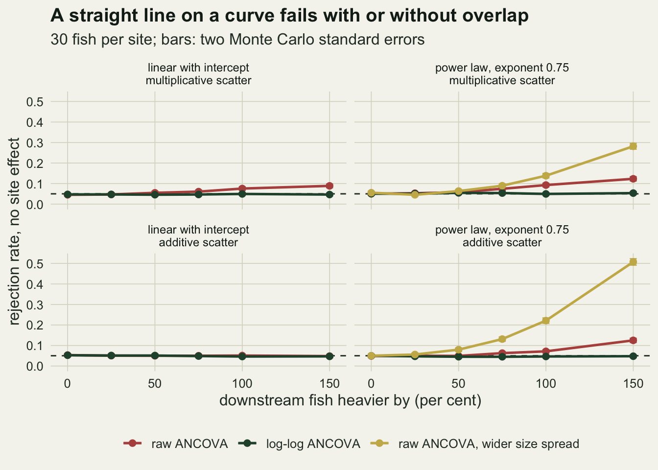
The ANCOVA figure is the part of this post the formula cannot supply. It is also a narrower result than the ratio figure: two truths, one intercept share, one exponent, two size spreads, and no claim that other curves behave the same way.
A real effect, reported backwards
The last case gives the downstream site a real effect: at any given body mass its fish carry a fixed percentage more liver. The size gap stays at 30 per cent and the intercept at 30 per cent of the mean, with multiplicative scatter: the corner of the grid where the null rejection rate was highest, so this is the strong end of the problem. The rates below count one-sided significant results in each direction at the two-sided five per cent level, so a significant ratio result in the wrong direction is counted as what it is.
The expected ratios are equal when (1 + effect)(b + a E[1/X2]) = b + a E[1/X1], which gives the effect size at which the ratio test has no expected signal at all.
eff_set <- c(0, 0.02, 0.04, 0.06, 0.08, 0.1, 0.12, 0.15)
set.seed(9304)
rev_tab <- do.call(rbind, lapply(eff_set, function(ef) {
  ts <- four_tests(draw_sites(n_rep, 0.3, 0.3, "mult", effect = ef))
  data.frame(effect = ef,
             ratio_down = mean(ts[, 1] < -crit2), ratio_up = mean(ts[, 1] > crit2),
             ancova_up = mean(ts[, 3] > crit3), log_log_up = mean(ts[, 4] > crit3),
             ancova_down = mean(ts[, 3] < -crit3))
}))
rv <- function(ef, col) rev_tab[rev_tab$effect == ef, col]
a3 <- icept_for(0.3)
inv1 <- exp(-mu_log + sd_log^2 / 2); inv2 <- exp(-(mu_log + log(1.3)) + sd_log^2 / 2)
eff_zero <- (b_liver + a3 * inv1) / (b_liver + a3 * inv2) - 1
The mean ratios cross at a true excess of 7.6 per cent. Below that the ratio test points the wrong way. With a true 4 per cent excess the ratio test declares the downstream livers significantly smaller in 21.7 per cent of studies and significantly larger in 0.03 per cent, while the log-log ANCOVA finds the real, positive effect in 19.2 per cent. At an 8 per cent excess, just past the crossing, the ratio test is nearly blind (1.9 per cent wrong way, 3.4 per cent right way) and the log-log ANCOVA detects the effect in 59.5 per cent. The raw ANCOVA gave a wrong-direction significant result in at most 2.33 per cent of studies at any effect size, and that maximum is at no effect, where half of the nominal five per cent falls in each tail.
rev_long <- data.frame(effect = rep(rev_tab$effect, 3),
  rate = c(rev_tab$ratio_down, rev_tab$ratio_up, rev_tab$log_log_up),
  what = factor(rep(c("ratio: downstream significantly lower",
                      "ratio: downstream significantly higher",
                      "log-log ANCOVA: downstream significantly higher"), each = length(eff_set)),
                levels = c("ratio: downstream significantly lower",
                           "ratio: downstream significantly higher",
                           "log-log ANCOVA: downstream significantly higher")))
ggplot(rev_long, aes(100 * effect, rate, colour = what)) +
  geom_vline(xintercept = 100 * eff_zero, colour = te_body, linetype = "dashed", linewidth = 0.5) +
  geom_line(linewidth = 0.9) + geom_point(size = 2) +
  scale_colour_manual(values = c(te_rust, te_gold, te_forest), name = NULL) +
  scale_y_continuous(limits = c(0, 1)) +
  guides(colour = guide_legend(ncol = 1)) +
  labs(x = "true downstream liver excess at a given body mass (per cent)",
       y = "share of studies",
       title = "The ratio reports the effect with the wrong sign",
       subtitle = "downstream fish 30 per cent heavier; dashed: where the mean ratios are equal") +
  theme_datasheet() + theme(legend.position = "bottom")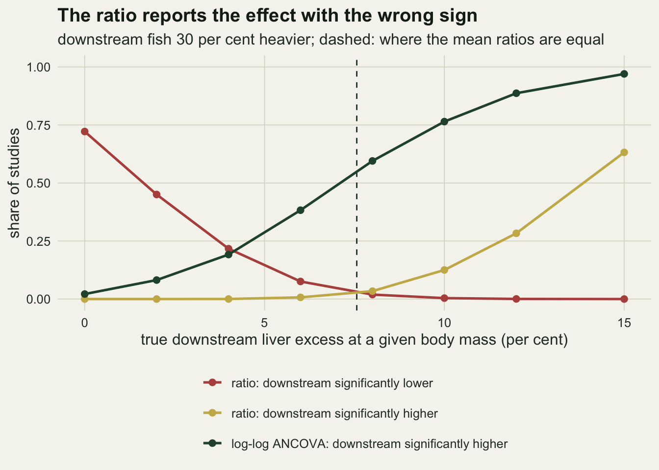
For an ecotoxicology report this is the uncomfortable case. A contaminant that enlarges the liver by a few per cent at a given size, at a site where the fish grow bigger, can produce a published, significant decrease in the hepatosomatic index. The crossing point depends on the intercept and the size gap, so there is no general effect size below which the reversal happens; the formula above gives it for any pair of values, and the intercept is the one that has to be estimated from the data.
What to report
Report the relationship before the index. A scatter of the organ mass against body mass with both sites marked shows at once whether a line through zero is a fair description, and the intercept of a pooled fit, as a share of the mean response, says how much a ratio will be distorted. In the grid above the ratio test held its nominal level at every size gap only when that share was zero.
Test the site effect with body size as a covariate, on the log scale by default. In this post the log-log ANCOVA held its level in every setting, including the linear truth it does not fit exactly, and the raw ANCOVA failed on a curved truth more often as the size gap grew, with or without overlap. Give the common slope with its interval and check that the slopes do not differ between sites before reading the site term, following the order set out in the isometry post.
Check the shape before trusting the site term, and do it on the scale of the model: plot the residuals against body mass for each site, or look at the log-log scatter, and look for a bend. Overlap does not protect a raw ANCOVA with the wrong shape; in this post it rejected more null datasets with most fish overlapping than with almost none. What non-overlap does is remove the fish that would reveal the bend, so a small overlap makes the shape check weaker, not the model safer. State the overlap in numbers as well (the share of fish in one site that fall inside the size range of the other is enough). If it is small, say that the site effect rests on the fitted line outside the data, show the fitted lines over the data, and expect the interval to be wide: the power to detect a real effect fell from 85.0 to 31.2 per cent between full overlap and a doubling of mass in the setting above.
If an index has to be reported, because a monitoring protocol or an older series demands it, report it next to the ANCOVA and not instead of it. Where the two disagree in sign, the ANCOVA is the one that compares fish of the same size.
Honest limits
The truth throughout has one common slope for both sites. A real contaminant can change the slope as well as the elevation, and then the site effect in an ANCOVA depends on the body size at which it is evaluated; no single number, ratio or adjusted mean, describes it. The slope test comes first for that reason, and nothing here measures how often it misses a slope difference at 30 fish per site.
Body mass is measured without error. A covariate with measurement error attenuates the within-site slope, and a biased slope leaves part of the size gap unadjusted, so ANCOVA with an error-laden covariate can find a spurious site effect for the same reason the ratio does. The size of that effect grows with the size gap and the measurement error, and it is not in these numbers.
The size distributions are log-normal with the same spread at both sites, and the gap is a shift in the median. Sites that differ in the spread of sizes, or in their shape, change the value of E[1/X] at each site and so the ratio bias; the closed form extends to any log-normal pair, but other distributions need their own moments.
The wrong-shape result rests on two truths, one intercept share and two size spreads. The weight split explains the asymmetry at one gap and one spread, with noise-free samples; it was not repeated across the grid. The log-log ANCOVA held on the linear truth because its equal weights put the pooled slope near the secant, rather than because the log curve is straight. With an intercept that is a larger share of the response, a gap of several doublings, or sites with different size spreads on the log scale (which would unbalance the weights), it may fail, and the grid does not show where. The raw ANCOVA’s failure on the power law depends on the exponent chosen, 0.75; an exponent nearer one bends less, and was not run.
The organ mass is not part of the body mass here. In real data the liver is inside the body weight, which adds a small built-in dependence between numerator and denominator; using body mass without the organ removes it, and for a liver of one or two per cent of body mass the dependence is small, but for gonads late in the season it need not be.
Finally, the analysis compares two sites with 30 fish each. That is a design with one site per treatment, so any difference, real or spurious, is a difference between two places and not an effect of the outfall; the pseudoreplication problem is untouched by the choice between a ratio and an ANCOVA.
References
Packard GC, Boardman TJ 1988 Physiological Zoology 61(1):1-9 (10.1086/physzool.61.1.30163730)
Kronmal RA 1993 Journal of the Royal Statistical Society Series A 156(3):379-392 (10.2307/2983064)
Garcia-Berthou E 2001 Journal of Animal Ecology 70(4):708-711 (10.1046/j.1365-2656.2001.00524.x)