SMA or OLS for a scaling exponent?

The standardised major axis is ordinary least squares divided by the correlation: why that identity makes SMA steeper, and when it is the unbiased choice.

Once you have logged both variables, you still have to draw a line through them, and allometry has two competing conventions. Ordinary least squares minimises vertical distances and treats the x variable as known. The standardised major axis, also called the reduced major axis, treats the two variables symmetrically and almost always gives a steeper slope.

The literature on which to use is long and not entirely friendly. Most of it can be compressed into one identity and one condition, both of which you can verify in a few lines of R. This post derives them by measurement, then shows what happens when the condition fails.

The identity

Write r for the correlation between the logged variables. The ordinary least squares slope is sd(y) / sd(x) multiplied by r. The standardised major axis slope drops that multiplier:

sma_slope <- function(x, y) sign(cor(x, y)) * sd(y) / sd(x)

deming_slope <- function(x, y, delta) {
  sxx <- var(x); syy <- var(y); sxy <- cov(x, y)
  (syy - delta * sxx + sqrt((syy - delta * sxx)^2 + 4 * delta * sxy^2)) / (2 * sxy)
}

set.seed(380)
n_sp <- 300
x_obs <- rnorm(n_sp, 3, 0.8)
y_obs <- 0.75 * x_obs + rnorm(n_sp, 0, 0.45)

b_ols <- unname(coef(lm(y_obs ~ x_obs))[2])
b_sma <- sma_slope(x_obs, y_obs)
r_obs <- cor(x_obs, y_obs)
c(ols = b_ols, sma = b_sma, r = r_obs,
  ols_over_r = b_ols / r_obs,
  gap = abs(b_sma - b_ols / r_obs))

         ols          sma            r   ols_over_r          gap 
7.776958e-01 9.453785e-01 8.226290e-01 9.453785e-01 9.992007e-16 

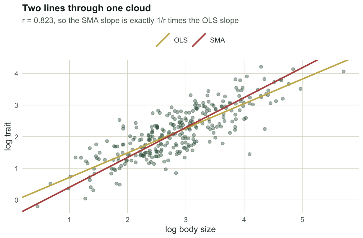
The standardised major axis slope is the ordinary least squares slope divided by the correlation, and the two agree to 1.0e-15, which is machine precision rather than approximation. On these data the correlation is 0.823, so the standardised major axis runs 21.6 percent steeper.

That is worth sitting with. The gap between the two exponents carries no biological information at all. It is a function of the scatter and nothing else.

rr <- c(0.99, 0.95, 0.90, 0.80, 0.70, 0.50)
data.frame(correlation = rr, sma_over_ols = round(1 / rr, 3))

  correlation sma_over_ols
1        0.99        1.010
2        0.95        1.053
3        0.90        1.111
4        0.80        1.250
5        0.70        1.429
6        0.50        2.000

At a correlation of 0.9, a perfectly respectable value for an interspecific dataset, the standardised major axis exponent is 11.1 percent above the least squares one. Papers have argued over exponent differences smaller than that.

Figure 1: The same logged data with both lines. The standardised major axis passes through the same centroid but tilts towards the axis of greatest spread, and the gap widens as the scatter grows.

The standardised major axis is a Deming fit in disguise

A Deming regression asks you to supply delta, the ratio of the error variance in y to the error variance in x, and then minimises a weighted perpendicular distance. Set delta to the ratio of the two observed variances and the algebra collapses.

delta_obs <- var(y_obs) / var(x_obs)
c(sma = b_sma,
  deming_at_var_ratio = deming_slope(x_obs, y_obs, delta_obs),
  gap = abs(b_sma - deming_slope(x_obs, y_obs, delta_obs)))

                sma deming_at_var_ratio                 gap 
       9.453785e-01        9.453785e-01        2.220446e-16 

Again exact, to 2.2e-16. So the standardised major axis is not an assumption-free method. It is a Deming fit that has quietly assumed the error variance ratio equals the total variance ratio of the data, which is to say it has assumed both variables are measured with the same relative precision. Nobody is asked to defend that assumption because nobody is asked to state it.

When is that assumption right?

Set up a structural model with known parts. Let the true log body size be x_t, let the true relationship be y_t = b * x_t, and let each variable pick up its own independent error. Then ask which estimator recovers b.

The algebra gives a sharp answer. The observed variances are var(x) = var(x_t) + var(e_x) and var(y) = b^2 * var(x_t) + var(e_y), so the standardised major axis estimates the square root of their ratio. That equals b exactly when var(e_y) = b^2 * var(e_x), and not otherwise.

b_str <- 0.75
n_str <- 400
n_mc <- 2000

run_config <- function(sd_ex, sd_ey, seed) {
  set.seed(seed)
  out <- t(vapply(seq_len(n_mc), function(i) {
    xt <- rnorm(n_str, 3, 0.8)
    x <- xt + rnorm(n_str, 0, sd_ex)
    y <- b_str * xt + rnorm(n_str, 0, sd_ey)
    c(unname(coef(lm(y ~ x))[2]),
      sma_slope(x, y),
      deming_slope(x, y, sd_ey^2 / sd_ex^2))
  }, numeric(3)))
  colMeans(out)
}

cfg <- list(c(0.30, 0.225), c(0.30, 0.300), c(0.30, 0.100), c(0.30, 0.450))
tab <- do.call(rbind, lapply(seq_along(cfg), function(k) {
  m <- run_config(cfg[[k]][1], cfg[[k]][2], 4380 + k)
  data.frame(sd_ex = cfg[[k]][1], sd_ey = cfg[[k]][2],
             err_ratio = round(cfg[[k]][2]^2 / cfg[[k]][1]^2, 3),
             ols = round(m[1], 4), sma = round(m[2], 4),
             deming_true = round(m[3], 4))
}))
tab

  sd_ex sd_ey err_ratio    ols    sma deming_true
1   0.3 0.225     0.563 0.6580 0.7506      0.7507
2   0.3 0.300     1.000 0.6571 0.7851      0.7499
3   0.3 0.100     0.111 0.6575 0.7122      0.7505
4   0.3 0.450     2.250 0.6579 0.8787      0.7508

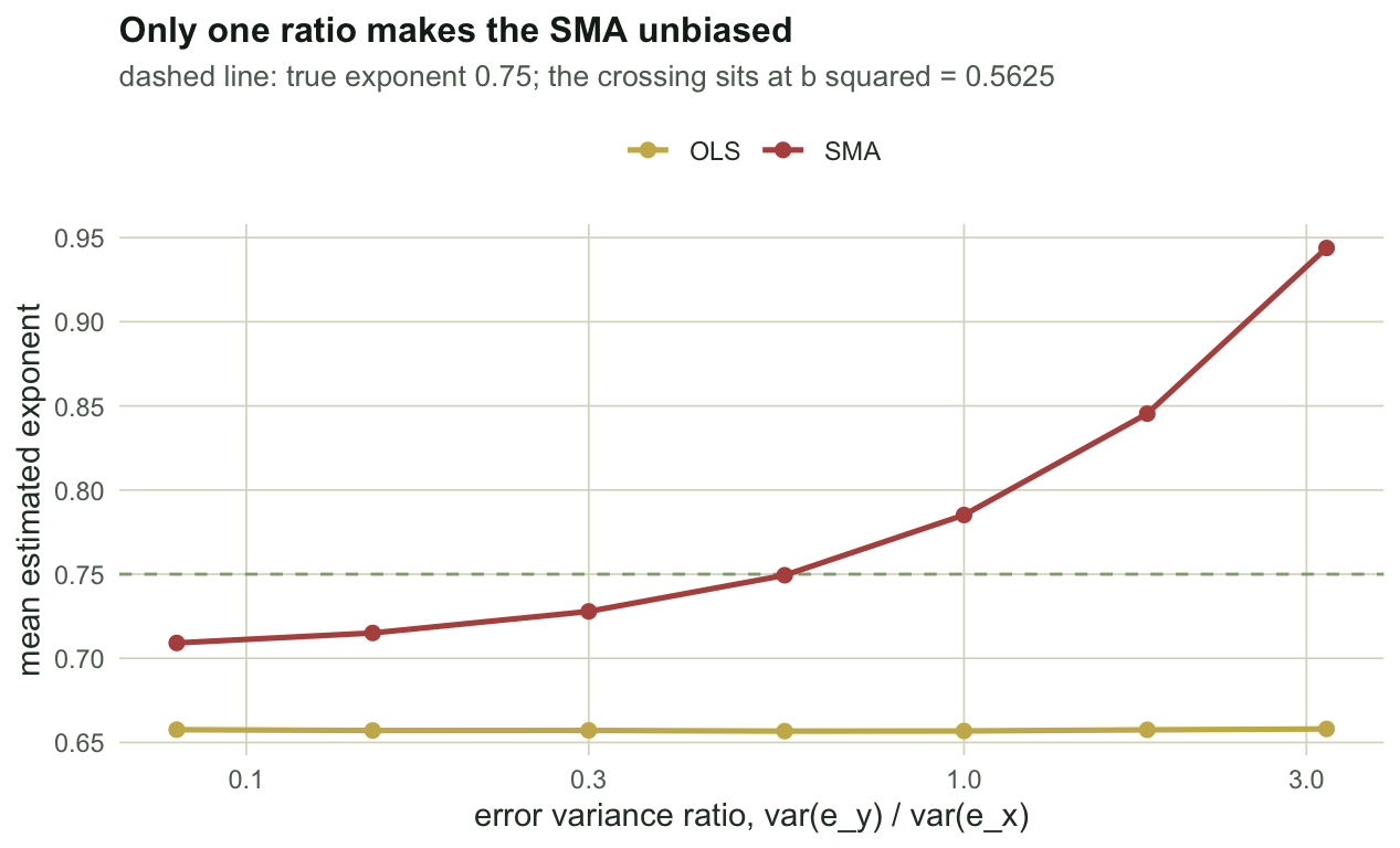
The critical ratio is b^2, which for a true exponent of 0.75 is 0.5625. The first row sits on it, and the standardised major axis returns 0.7506 against a truth of 0.75. Move off it and the estimate moves with it: equal error variances give 0.7851, a precise y variable gives 0.7122, and a noisy y variable gives 0.8787. Least squares sits at about 0.658 throughout, attenuated by the x error in the usual way, and Deming with the true ratio recovers the exponent in all four rows.

So the standardised major axis is not a fix for measurement error. It is a fix for one specific measurement error ratio, and it is biased in a knowable direction everywhere else: too steep when y is noisy relative to x, too shallow when x is the noisy one.

Figure 2: Mean estimated exponent across a sweep of error variance ratios, with the x error held fixed. The standardised major axis crosses the truth exactly once, at a ratio equal to the squared exponent.

Equation error breaks the condition on its own

There is a second source of scatter that has nothing to do with instruments. Two species of the same body mass genuinely differ in metabolic rate, and no amount of careful measurement removes that. Warton and colleagues call this equation error, to distinguish it from measurement error, and it lands entirely in the y variable.

Notice what that does to the condition. Equation error adds to var(e_y) while contributing nothing to var(e_x). If your x variable is measured well, as body mass usually is, the ratio sits far above b^2 and the standardised major axis runs steep. Take the limiting case where x is measured perfectly:

set.seed(3801)
xt <- rnorm(n_str, 3, 0.8)
x_clean <- xt
y_eqn <- b_str * xt + rnorm(n_str, 0, 0.30)
c(true_b = b_str,
  ols = unname(coef(lm(y_eqn ~ x_clean))[2]),
  sma = sma_slope(x_clean, y_eqn))

   true_b       ols       sma 
0.7500000 0.7558680 0.8376817 

With no error in x at all, least squares is the correct estimator and returns 0.756, while the standardised major axis returns 0.838. Switching to the symmetric method because “both variables are biological” has made the answer worse, not safer.

Where to go next

The choice of line is a choice of error model, and the data cannot make it for you. Three practical positions:

If your x variable is measured much more precisely than the scatter in y, and the scatter is mostly biological, ordinary least squares estimates the relationship you want. If you are describing the joint spread of two traits rather than predicting one from the other, the standardised major axis is a reasonable descriptive summary, and its symmetry is a genuine advantage: it gives the same line whichever variable you put on the x axis. If you actually know something about the two error variances, from repeated measurements or from instrument specifications, Deming with that ratio dominates both.

What you should not do is pick the method that gives the exponent closest to the value you expected. The gap between the two lines is 1/r, and it is available to be exploited in either direction.

Honest limits

Everything above is about the point estimate. Intervals are a separate problem: the sampling distribution of the standardised major axis slope is skewed, and its confidence interval is not the usual symmetric Wald form. The condition var(e_y) = b^2 * var(e_x) is also not testable from a single bivariate sample, because the observed variances confound signal and error. That is the same wall the errors-in-variables literature runs into everywhere: a ratio has to come from outside the data.

References

Warton, Wright, Falster, Westoby 2006 Biological Reviews 81(2):259-291 (10.1017/S1464793106007007)

Warton, Weber 2002 Biometrical Journal 44(2):161-174 (10.1002/1521-4036(200203)44:2<161::AID-BIMJ161>3.0.CO;2-N)

Xiao, White, Hooten, Durham 2011 Ecology 92(10):1887-1894 (10.1890/11-0538.1)

Related tutorials

• Errors in variables and Deming regression - the general two-error line fit that the SMA is a special case of.
• Allometry and log-log regression in R - getting onto the log scale and back off it again.
• Measurement error and regression dilution - why the least squares slope attenuates, and by how much.
• Testing isometry and comparing slopes - inference once the line is chosen.