Back-transforming a log-scale model

Exponentiating a log-scale biomass equation returns the median tree, not the mean one, so stand totals come out low. Two corrections, and when each fails.

You harvest and weigh a couple of hundred trees, fit lm(log(mass) ~ log(diameter)), and the fit looks excellent: the points lie along a straight line, the residuals are an even band. Then you apply the equation to the inventory, exponentiate each prediction, and add them up. The stand total that comes back is too low, and it is too low by a percentage that more fieldwork will not remove.

The exponentiated line is not estimating what most people assume. It estimates the conditional median of mass at a given diameter. Mass at a given diameter is right-skewed, so the median sits below the mean, and a total is a sum of means. The size of the gap is set by the residual spread on the log scale, and hardly at all by anything else: not, once the calibration sample is more than a handful of trees, by the sample size, not by the R squared, not by how carefully the trees were weighed.

Fitting the equation and applying the standard correction to it is the subject of Allometry and log-log regression in R. This post starts where that one stops. It pins the bias down against a truth the simulation knows exactly, shows what the correction leaves behind on a single stand, then breaks the usual correction on purpose. It closes with the case that needs no fix at all, because a log link and a logged response are the pair most often confused.

The exponentiated line is a median

Simulate a stand where the truth is known. Mass follows a power law in diameter with a multiplicative error, which is the standard model behind almost every published biomass equation.

library(ggplot2)

te_paper  <- "#f5f4ee"
te_ink    <- "#16241d"
te_body   <- "#2c3a31"
te_forest <- "#275139"
te_rust   <- "#b5534e"
te_gold   <- "#c9b458"
te_line   <- "#dad9ca"

theme_datasheet <- function() {
  theme_minimal(base_size = 12) +
    theme(plot.background  = element_rect(fill = te_paper, colour = NA),
          panel.background = element_rect(fill = te_paper, colour = NA),
          panel.grid.major = element_line(colour = te_line, linewidth = 0.3),
          panel.grid.minor = element_blank(),
          text             = element_text(colour = te_body),
          plot.title       = element_text(colour = te_ink, face = "bold"),
          axis.text        = element_text(colour = te_body))
}

set.seed(8213)
n_stem <- 400
a_true <- 0.088
b_true <- 2.42
s_true <- 0.45                      # residual SD on the log scale

dbh  <- exp(rnorm(n_stem, log(24), 0.5))
mass <- a_true * dbh^b_true * exp(rnorm(n_stem, 0, s_true))

fit   <- lm(log(mass) ~ log(dbh))
s_hat <- summary(fit)$sigma
round(c(intercept = unname(coef(fit)[1]), slope = unname(coef(fit)[2]),
        resid_sd = s_hat), 3)

intercept     slope  resid_sd 
   -2.469     2.434     0.464 

The fitted exponent is 2.434 against a true 2.42, and the log-scale residual standard deviation is 0.464. Nothing is wrong with this fit. Now back-transform it and ask two separate questions of the answer: does it split the trees in half, and does it reproduce their average.

naive <- exp(fitted(fit))                       # exponentiated fitted line
share_below <- mean(mass < naive)
tot_true    <- sum(mass)
tot_naive   <- sum(naive)
round(c(share_below_line = share_below,
        true_total_t     = tot_true / 1000,
        naive_total_t    = tot_naive / 1000,
        shortfall_pct    = 100 * (1 - tot_naive / tot_true)), 3)

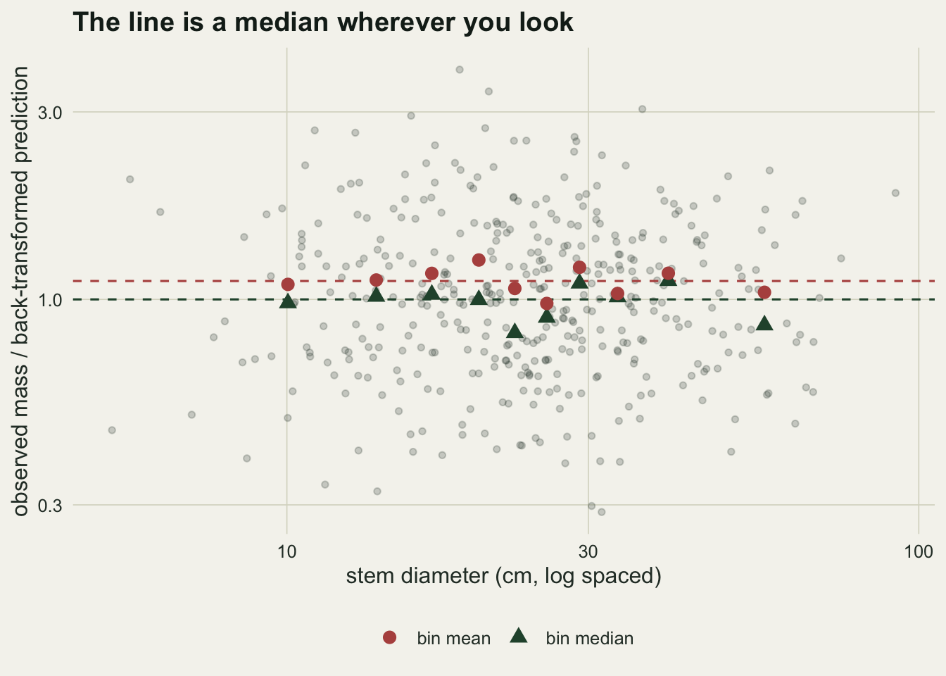
share_below_line     true_total_t    naive_total_t    shortfall_pct 
           0.492          167.445          151.387            9.590 

49.2 per cent of the trees weigh less than the line predicts for them. As a median the back-transformation is doing its job, landing where it should. As a mean it is 9.6 per cent short, which on this stand is 16.1 tonnes of missing biomass out of 167.4.

Both statements are about the same line. That is the whole difficulty: a curve can be an excellent estimate of the typical tree and a poor estimate of the average tree at the same time, and only the second one adds up.

ratio <- mass / naive
dbin  <- cut(dbh, breaks = quantile(dbh, seq(0, 1, length.out = 11)),
             include.lowest = TRUE)
bin_dbh  <- tapply(dbh, dbin, mean)
bin_med  <- tapply(ratio, dbin, median)
bin_mean <- tapply(ratio, dbin, mean)
binned <- rbind(
  data.frame(dbh = bin_dbh, y = bin_med,  stat = "bin median"),
  data.frame(dbh = bin_dbh, y = bin_mean, stat = "bin mean"))

ggplot(binned, aes(dbh, y)) +
  geom_point(data = data.frame(dbh = dbh, y = ratio), colour = te_body,
             alpha = 0.22, size = 1.3) +
  geom_hline(yintercept = 1, colour = te_forest, linetype = "dashed") +
  geom_hline(yintercept = exp(s_hat^2 / 2), colour = te_rust,
             linetype = "dashed") +
  geom_point(aes(colour = stat, shape = stat), size = 3) +
  scale_colour_manual(values = c(te_rust, te_forest)) +
  scale_x_log10() +
  scale_y_log10() +
  labs(x = "stem diameter (cm, log spaced)",
       y = "observed mass / back-transformed prediction",
       colour = NULL, shape = NULL,
       title = "The line is a median wherever you look") +
  theme_datasheet() +
  theme(legend.position = "bottom")

Figure 1: Each tree’s mass divided by its own back-transformed prediction, summarised as a mean and a median within ten diameter bins, against the two horizontal references the fit implies.

Split the trees into diameter deciles and look inside each one. Forty trees is not many, so the bin statistics scatter: the lowest bin median sits 18 per cent below the lower line. What survives the scatter is the comparison within a bin: the mean ratio exceeds the median ratio in 10 bins out of ten, by an average of 0.130 against the 0.114 that separates the two dashed lines. Neither set drifts with diameter, which is what makes a single multiplier the right kind of repair. That multiplier is the upper dashed line, at 1.114.

More trees will not help

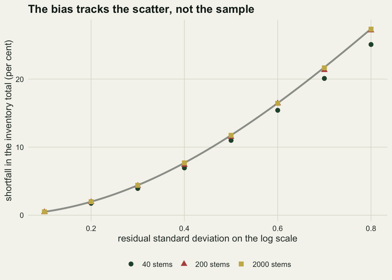
The obvious response to a total that is 9.6 per cent low is to suspect the sample. Fit the equation on more stems, the reasoning goes, and the estimate will settle down. It will: the coefficients settle down beautifully, and the shortfall does not settle anywhere near zero.

The quantity that governs the shortfall is the residual spread. Under lognormal residuals the ratio of the median to the mean at any diameter is exp(-sigma^2/2), and there is no n in that expression. So run the simulation the way the fieldwork runs: fit the equation on n harvested stems, apply it to a standing inventory those stems are not part of, and score it against the expected total of that inventory, which the generating model states exactly. Then cross a grid of residual spreads with a grid of calibration sample sizes.

set.seed(4021)
inv_dbh <- exp(rnorm(2000, log(24), 0.5))     # the standing inventory
inv_lgd <- log(inv_dbh)
inv_mu  <- a_true * inv_dbh^b_true            # expected mass before the error

true_mult <- function(s, shape = "normal") {  # E[exp(residual)]
  if (shape == "normal") return(exp(s^2 / 2))
  k <- 0.5
  a <- s / sqrt(k)
  if (shape == "right-skewed") exp(-a * k) * (1 - a)^(-k)
  else                         exp( a * k) * (1 + a)^(-k)
}

one_stand <- function(n, s) {
  d <- exp(rnorm(n, log(24), 0.5))
  y <- a_true * d^b_true * exp(rnorm(n, 0, s))
  b <- unname(coef(lm(log(y) ~ log(d))))
  sum(exp(b[1] + b[2] * inv_lgd)) / (sum(inv_mu) * true_mult(s))
}

set.seed(51)
n_rep  <- 4000
design <- expand.grid(s = seq(0.1, 0.8, by = 0.1), n = c(40, 200, 2000))
cells  <- mapply(function(n, s) {
  v <- replicate(n_rep, one_stand(n, s))
  c(100 * (1 - mean(v)), 100 * sd(v) / sqrt(n_rep))
}, design$n, design$s)
design$shortfall <- cells[1, ]
design$mc_se     <- cells[2, ]

with(design, round(tapply(shortfall, list(s, n), mean), 2))

       40   200  2000
0.1  0.51  0.46  0.50
0.2  1.75  1.93  1.98
0.3  3.93  4.31  4.39
0.4  6.95  7.39  7.68
0.5 10.99 11.51 11.74
0.6 15.42 16.43 16.43
0.7 20.10 21.32 21.65
0.8 25.08 27.15 27.33

row_spread <- max(tapply(design$shortfall, design$s, function(v) diff(range(v))))
round(c(widest_gap_across_n  = row_spread,
        range_across_sigma   = diff(range(design$shortfall)),
        mc_se_smallest_sigma = max(design$mc_se[design$s == 0.1])), 3)

 widest_gap_across_n   range_across_sigma mc_se_smallest_sigma 
               2.252               26.877                0.041 

Read down the right-hand column and the shortfall runs from about half a per cent to more than a quarter of the biomass; across the whole table it swings 27 percentage points, driven by the residual spread alone. Read across a row and the widest disagreement between the three sample sizes anywhere in the table is 2.3 points, and it is not the disagreement anyone was hoping for. From the 0.2 row down, the 40 stem column sits below the other two, because the coefficients from a small calibration sample carry estimation variance of their own, which inflates exp(fitted) when the equation is applied and so conceals part of the bias. In the 0.1 row the three columns differ by less than a tenth of a point, against a Monte Carlo standard error of up to 0.041 on those cells, so that row settles nothing. The inflation shrinks as the calibration sample grows, so adding trees moves the shortfall towards its asymptote: it makes the number slightly worse.

theory <- data.frame(s = seq(0.1, 0.8, length.out = 200))
theory$shortfall <- 100 * (1 - exp(-theory$s^2 / 2))

design$stems <- factor(design$n, labels = c("40 stems", "200 stems",
                                            "2000 stems"))

ggplot(design, aes(s, shortfall)) +
  geom_line(data = theory, colour = te_body, linewidth = 1.1, alpha = 0.5) +
  geom_point(aes(colour = stems, shape = stems), size = 2.6) +
  scale_colour_manual(values = c(te_forest, te_rust, te_gold)) +
  labs(x = "residual standard deviation on the log scale",
       y = "shortfall in the inventory total (per cent)",
       colour = NULL, shape = NULL,
       title = "The bias tracks the scatter, not the sample") +
  theme_datasheet() +
  theme(legend.position = "bottom")

Figure 2: Mean shortfall of the naive inventory total across 4000 simulated calibration samples per cell, against the log-scale residual spread, for three calibration sample sizes.

The grey curve is 100 * (1 - exp(-sigma^2/2)), drawn from the formula rather than from the simulation, and the two larger sample sizes lie along it. This is why a tight equation fitted to one species on one site can be back-transformed carelessly and lose almost nothing, while a mixed-species equation with the scatter you actually meet in the field loses close to a tenth of the stand, and would lose the same tenth if it had been fitted to every tree in the country.

Two corrections, and the scatter they leave

If the log-scale residuals are normal, the fix is a single multiplier. Baskerville’s factor exp(sigma^2/2) is the mean of a lognormal whose median is one, and Duan’s smearing estimator reaches the same place without the distributional assumption, by averaging exp(residual) over the fitted residuals. Both are one line, and both are derived in the allometry post linked above. The question that post does not ask is how much of the error a multiplier actually removes from one stand.

cf_lnorm  <- exp(s_hat^2 / 2)
cf_smear  <- mean(exp(residuals(fit)))
round(c(lognormal_factor = cf_lnorm,
        smearing_factor  = cf_smear,
        lognormal_total_t = tot_naive * cf_lnorm / 1000,
        smearing_total_t  = tot_naive * cf_smear / 1000,
        true_total_t      = tot_true / 1000), 4)

 lognormal_factor   smearing_factor lognormal_total_t  smearing_total_t 
           1.1138            1.1130          168.6158          168.4868 
     true_total_t 
         167.4448 

On this stand the two multipliers agree to 0.001, and both take the total from 9.6 per cent short to 168.6 and 168.5 tonnes against a true 167.4, errors of 0.7 and 0.6 per cent. That is one stand, and one stand is an illustration rather than a result. Repeat the whole exercise instead, scoring each simulated stand against its own realised total, which is the comparison the paragraph above just made.

one_replicate <- function() {
  d <- exp(rnorm(n_stem, log(24), 0.5))
  y <- a_true * d^b_true * exp(rnorm(n_stem, 0, s_true))
  f <- lm(log(y) ~ log(d))
  p <- sum(exp(fitted(f)))
  c(naive     = p / sum(y),
    lognormal = p * exp(summary(f)$sigma^2 / 2) / sum(y),
    smearing  = p * mean(exp(residuals(f))) / sum(y))
}

set.seed(4471)
err <- 100 * (replicate(4000, one_replicate()) - 1)
round(rbind(mean_error_pct = rowMeans(err),
            lower_2.5      = apply(err, 1, quantile, 0.025),
            upper_97.5     = apply(err, 1, quantile, 0.975)), 2)

                naive lognormal smearing
mean_error_pct  -9.40      0.24     0.19
lower_2.5      -15.26     -6.05    -6.00
upper_97.5      -4.05      6.06     6.01

round(c(share_within_1_pc = mean(abs(err["lognormal", ]) < 1)), 3)

share_within_1_pc 
            0.294 

Across 4000 stands of the same size and spread the naive total is on average 9.4 per cent short, and correcting it moves the average error to 0.24 per cent, a residue 39 times smaller than the shortfall it replaced and pointing the other way. What the correction does not touch, and was never going to, is the scatter: the middle 95 per cent of corrected totals still runs from 6.0 per cent below the truth to 6.1 per cent above, and only 29 stands in a hundred land within one per cent of it. The worked stand above is one of those; a different seed would have given a corrected total several per cent out in either direction, with no bias to blame for it. What a multiplier buys is a total that is right on average, not a total that is right.

There is no reason to prefer one factor over the other here, which is exactly why the choice looks unimportant until the residuals stop being normal.

Where the parametric factor breaks

Residuals on the log scale are not always symmetric. A biomass sample that mixes species, or that catches a handful of stems with unusually dense wood or an unusually heavy crown load, has a long right tail on the log scale: most trees a little under the line, a few well over it. That is a different distribution with the same standard deviation, and exp(sigma^2/2) does not know the difference, because the standard deviation is all it is given.

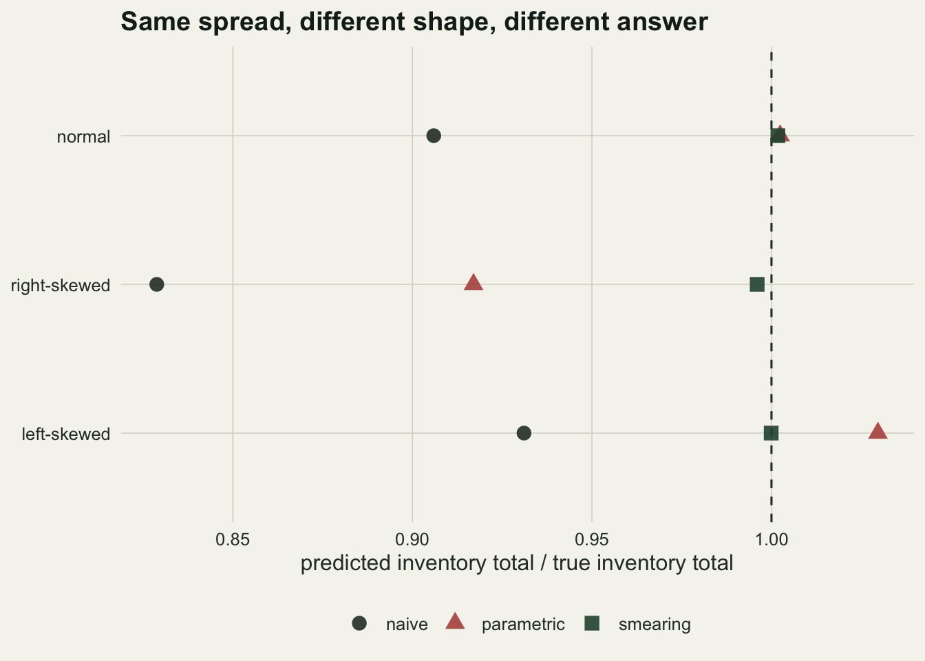
The following draws log-scale residuals from a shifted gamma, once skewed right and once skewed left, with the spread held at 0.45 in every case, so the parametric factor sees the same standard deviation whichever shape it is handed. Each calibration sample is again applied to the same standing inventory and scored against its expected total, which true_mult() supplies for each shape in closed form.

draw_resid <- function(n, s, shape) {
  if (shape == "normal") return(rnorm(n, 0, s))
  k <- 0.5
  a <- s / sqrt(k)                       # so that the SD is s in every case
  g <- a * (rgamma(n, shape = k, rate = 1) - k)
  if (shape == "right-skewed") g else -g
}

one_shape <- function(shape) {
  d <- exp(rnorm(300, log(24), 0.5))
  y <- a_true * d^b_true * exp(draw_resid(300, s_true, shape))
  f <- lm(log(y) ~ log(d))
  b <- unname(coef(f))
  p <- sum(exp(b[1] + b[2] * inv_lgd))
  truth <- sum(inv_mu) * true_mult(s_true, shape)
  c(naive      = p / truth,
    parametric = p * exp(summary(f)$sigma^2 / 2) / truth,
    smearing   = p * mean(exp(residuals(f))) / truth)
}

set.seed(9902)
shapes <- c("normal", "right-skewed", "left-skewed")
sims <- lapply(shapes, function(sh) replicate(2000, one_shape(sh)))
names(sims) <- shapes
res <- t(vapply(sims, rowMeans, numeric(3)))
round(res, 3)

             naive parametric smearing
normal       0.906      1.002    1.002
right-skewed 0.829      0.917    0.996
left-skewed  0.931      1.030    1.000

Each entry is the predicted inventory total as a fraction of the true one, averaged over 2000 calibration samples. On normal residuals the parametric factor lands on 1.002 and smearing on 1.002, both effectively unbiased.

On the right-skewed residuals the parametric factor takes the total from 0.829 to 0.917. That closes 52 per cent of the gap, so barely half of it, and leaves the inventory 8.3 per cent short, which is almost the whole 9.4 per cent shortfall that the same factor removes cleanly in the first row of the table. It is not an error you would want in a carbon inventory. Smearing returns 0.996. The long right tail carries real mass that a formula reading only the standard deviation cannot see, and that the observed residuals can.

The left-skewed case runs the other way and is the more awkward one to explain to a reviewer, because the correction overshoots: 1.030 against a truth of one, an overestimate of 3.0 per cent, where smearing gives 1.000. A correction that is supposed to raise a total too low can push it too high if the shape assumption is wrong in that direction.

long <- data.frame(shape  = rep(rownames(res), times = 3),
                   method = rep(colnames(res), each = 3),
                   ratio  = as.vector(res))
long$shape  <- factor(long$shape, levels = rev(shapes))
long$method <- factor(long$method,
                      levels = c("naive", "parametric", "smearing"))

ggplot(long, aes(ratio, shape, colour = method, shape = method)) +
  geom_vline(xintercept = 1, linetype = "dashed", colour = te_body) +
  geom_point(size = 3.4, alpha = 0.9) +
  scale_colour_manual(values = c(te_body, te_rust, te_forest)) +
  labs(x = "predicted inventory total / true inventory total", y = NULL,
       colour = NULL, shape = NULL,
       title = "Same spread, different shape, different answer") +
  theme_datasheet() +
  theme(legend.position = "bottom")

Figure 3: Predicted inventory total as a fraction of the truth for three back-transformations, under three log-scale residual shapes with identical standard deviations.

Smearing costs nothing and is the safer default. It is not free of assumptions, only of the distributional one, and the two it keeps are in the honest limits below.

A log link is not a log transform

None of this applies to a generalised linear model with a log link, and the reason is worth stating precisely because the two situations look alike in the code.

In lm(log(y) ~ x) the transformation is applied to the data. The model is a statement about E[log(y)], and exp() of that is the geometric mean of y, which is the median whenever the log-scale residuals are symmetric. In glm(y ~ x, family = Gamma(link = "log")) the transformation is applied to the expectation. The model is a statement about log(E[y]), so exp() of the linear predictor is already the mean and there is nothing to put right.

set.seed(707)
d2  <- exp(rnorm(500, log(24), 0.5))
mu2 <- a_true * d2^b_true
y2  <- rgamma(500, shape = 5, rate = 5 / mu2)     # mean mu2, right-skewed

m_lm  <- lm(log(y2) ~ log(d2))
m_glm <- glm(y2 ~ log(d2), family = Gamma(link = "log"))

round(c(expected_total_t = sum(mu2) / 1000,
        lm_naive_t       = sum(exp(fitted(m_lm))) / 1000,
        lm_smeared_t     = sum(exp(fitted(m_lm))) *
                             mean(exp(residuals(m_lm))) / 1000,
        glm_total_t      = sum(fitted(m_glm)) / 1000), 2)

expected_total_t       lm_naive_t     lm_smeared_t      glm_total_t 
          216.63           195.58           217.03           217.16 

The expected total is 216.6 tonnes. The exponentiated linear model gives 195.6 before correction and 217.0 after it. The gamma GLM gives 217.2 with nothing applied to it at all, because fitted() on a GLM is already on the response scale, and for a log link that scale is the mean. The same holds for a Poisson or negative binomial count model with a log link.

So the trap is specific: it is the logged response, not the log link. If your workflow is a GLM and you want predicted values on the response scale, the questions worth your attention are the shape of the interval and where you park the other predictors, which is the subject of From GLM coefficients to predicted values in R.

Honest limits

The correction needs sigma, and sigma comes from the same fit whose predictions it is repairing. On a small calibration sample the residual standard deviation is itself uncertain, and because it enters through exp(sigma^2/2) that uncertainty is amplified: the factor is not a known constant and a total built on it deserves an interval that says so. The plug-in version used here is also not the only option: an exact small-sample estimator of a lognormal mean has been available since Finney’s work in the 1940s, and it differs from exp(sigma^2/2) by a little at the sample sizes a harvesting campaign can afford.

Smearing drops the distributional assumption and keeps a harder one. The residuals have to be exchangeable across the predictor range, because a single scalar multiplier is being averaged over all of them at once. If the log-scale scatter widens with diameter, which is common when small stems are weighed whole and large ones are subsampled, then the multiplier is too large for the small trees and too small for the large ones, and since the large trees carry the mass, the total inherits the error of the wrong end. In that situation the honest options are a size-dependent factor estimated within strata or a model that carries the variance function explicitly, not a scalar.

The other assumption smearing keeps is that averaging is enough. Its multiplier is a mean of exp() over the residuals, so the heavier the right tail, the more that mean depends on the few largest of them. Under the right-skewed residuals above the estimator is close to unbiased across calibration samples, at 0.996, but the median sample returns 0.968, some 3 per cent low, and the average is held up by the minority of samples that happen to contain one of the very large residuals. Unbiased across many campaigns is not the same as accurate on yours.

Finally, the whole problem is conditional on wanting a mean. Plenty of ecological questions want a median: the typical stem in a size class, or a ratio between two stands in which the factor cancels anyway. For those, exp(fitted) is the right answer and applying a correction to it is the error. The question to settle before reaching for a multiplier is which of the two quantities the next step in the analysis is going to add up.

References

Baskerville GL 1972 Canadian Journal of Forest Research 2(1):49-53 (10.1139/x72-009)

Duan N 1983 Journal of the American Statistical Association 78(383):605-610 (10.1080/01621459.1983.10478017)

Sprugel DG 1983 Ecology 64(1):209-210 (10.2307/1937343)

Finney DJ 1941 Journal of the Royal Statistical Society Series B 7(2):155-161 (10.2307/2983663)

Xiao X, White EP, Hooten MB, Durham SL 2011 Ecology 92(10):1887-1894 (10.1890/11-0538.1)

Related tutorials

• Allometry and log-log regression in R
• Checking an allometric analysis
• From GLM coefficients to predicted values in R
• SMA or OLS for a scaling exponent?