library(ggplot2)

te_paper  <- "#f5f4ee"
te_ink    <- "#16241d"
te_body   <- "#2c3a31"
te_forest <- "#275139"
te_rust   <- "#b5534e"
te_gold   <- "#c9b458"
te_line   <- "#dad9ca"

theme_datasheet <- function() {
  theme_minimal(base_size = 12) +
    theme(plot.background  = element_rect(fill = te_paper, colour = NA),
          panel.background = element_rect(fill = te_paper, colour = NA),
          panel.grid.major = element_line(colour = te_line, linewidth = 0.3),
          panel.grid.minor = element_blank(),
          text             = element_text(colour = te_body),
          plot.title       = element_text(colour = te_ink, face = "bold"),
          axis.text        = element_text(colour = te_body))
}

step   <- 1 / 96                        # fifteen minutes, expressed in days
tod    <- (seq_len(96) - 0.5) / 96      # time of day
c_sat  <- 9.0                           # saturation, mg/L, near 20 degrees C

# normalised light: a sine over a fourteen hour photoperiod, integrating to one
light <- pmax(sin(pi * (tod - 0.22) / 0.58), 0)
light <- light / (sum(light) * step)

# five days are integrated and the last one kept, so the series is on its
# repeating daily cycle and carries no start up transient
simulate_do <- function(gpp, er, k_gas, depth, c0 = 8.6, noise = 0, days = 5) {
  n <- 96 * days; lt <- rep(light, days)
  conc <- numeric(n); conc[1] <- c0
  for (i in 2:n)
    conc[i] <- conc[i - 1] + step * ((gpp * lt[i - 1] - er) / depth +
                                     k_gas * (c_sat - conc[i - 1]))
  conc[(n - 95):n] + rnorm(96, 0, noise)
}Stream metabolism from one oxygen logger
R
freshwater ecology
ecosystem fluxes
time series
ecology tutorial
One dissolved oxygen sensor gives whole stream production and respiration. On a deep, fast reach a correct model returns impossible fluxes a third of the time.
A dissolved oxygen sensor is left in a stream for a day, logging every fifteen minutes. Overnight the oxygen falls because everything in the reach is respiring; through the morning it climbs because the algae and biofilms are photosynthesising; all day it is being pulled towards saturation by exchange with the atmosphere. Fit those three processes to the curve and you have gross primary production and ecosystem respiration for the whole reach, from one instrument and no chambers.
That is the single station open channel method, and it is the standard way freshwater ecologists get whole ecosystem fluxes. The arithmetic is not in question. What this post measures is how much of the answer survives the geometry of the reach the sensor happens to be in, using data generated from the model itself, so the true fluxes are known and the model being fitted is exactly the model that made the data.
The site’s terrestrial counterpart, splitting net ecosystem exchange into production and respiration, extrapolates a night time respiration model into the day. The aquatic problem is different: all three processes act on one curve at once, and one of them is a physical gas exchange term with no terrestrial analogue.
The model
Oxygen concentration in a well mixed reach changes for three reasons.
Production adds oxygen in proportion to light, respiration removes it at a constant rate, and both are areal fluxes in grams of oxygen per square metre per day, so both are divided by mean depth to become concentration changes. Gas exchange moves the concentration towards saturation at a rate set by the reaeration coefficient, written here as a first order rate constant in units of one over days. Nothing else is in the model.
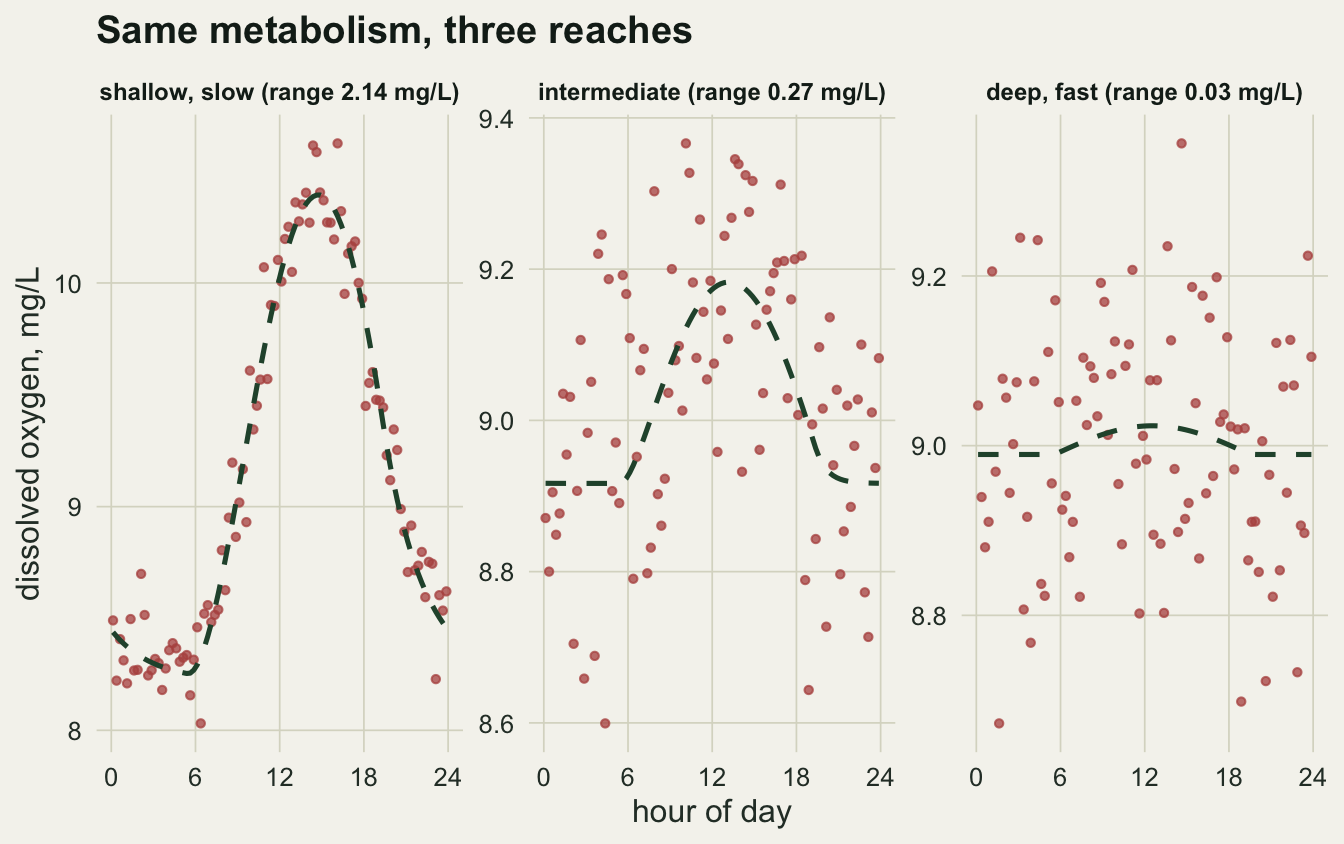
Three reaches carry the same biology: a shallow, slow, open stream, an intermediate one, and a deep, fast, turbulent river. Gross primary production and ecosystem respiration are identical in all three.
reaches <- data.frame(
  name  = c("shallow, slow", "intermediate", "deep, fast"),
  depth = c(0.4, 1.2, 3.0),
  k_gas = c(8, 25, 80))
gpp_true <- 3.0; er_true <- 2.5

swings <- sapply(seq_len(nrow(reaches)), function(i)
  diff(range(simulate_do(gpp_true, er_true, reaches$k_gas[i], reaches$depth[i]))))
reaches$diel_range <- round(swings, 3)
reaches
name depth k_gas diel_range
1 shallow, slow 0.4 8 2.139
2 intermediate 1.2 25 0.266
3 deep, fast 3.0 80 0.034Production is 3.0 and respiration 2.5 grams of oxygen per square metre per day everywhere, so the true production to respiration ratio is 1.20. The shallow reach is 0.4 m deep with a reaeration coefficient of 8 per day; the deep one is 3.0 m with a coefficient of 80 per day.
That same metabolism writes a 2.14 mg/L swing into the shallow reach and only 0.03 mg/L into the deep one. Depth dilutes the areal flux and reaeration erases what is left of it, so the signal available to the estimator is smaller by a factor of 62.9.
Fitting the curve
The estimator integrates the model forward from the first observed concentration and picks the production and respiration that minimise the squared difference from the logged series. The reaeration coefficient is held at its true value, which is the most generous assumption available.
fit_metab <- function(obs, k_gas, depth, start = c(5, 5)) {
  rss <- function(par) {
    conc <- numeric(96); conc[1] <- obs[1]
    for (i in 2:96)
      conc[i] <- conc[i - 1] + step * ((par[1] * light[i - 1] - par[2]) / depth +
                                       k_gas * (c_sat - conc[i - 1]))
    sum((obs - conc)^2)
  }
  o <- optim(start, rss, method = "Nelder-Mead",
             control = list(reltol = 1e-10, maxit = 2000))
  c(gpp = o$par[1], er = o$par[2])
}

set.seed(5220)
one_day <- simulate_do(gpp_true, er_true, reaches$k_gas[1], reaches$depth[1],
                       noise = 0.15)
round(fit_metab(one_day, reaches$k_gas[1], reaches$depth[1]), 3)
gpp er
2.839 2.305 On one day from the shallow reach the fit returns production and respiration within a few per cent of the truth. Three hundred days from each reach, all generated with the same true fluxes and the same sensor, give the distribution of what the method returns.
run_reach <- function(i, nrep = 300, seed) {
  set.seed(seed)
  out <- t(replicate(nrep, {
    obs <- simulate_do(gpp_true, er_true, reaches$k_gas[i], reaches$depth[i],
                       noise = 0.15)
    fit_metab(obs, reaches$k_gas[i], reaches$depth[i])
  }))
  data.frame(reach = reaches$name[i], gpp = out[, 1], er = out[, 2])
}
sims <- do.call(rbind, lapply(seq_len(nrow(reaches)),
                              function(i) run_reach(i, seed = 5300 + i)))

summary_tab <- do.call(rbind, lapply(reaches$name, function(nm) {
  d <- sims[sims$reach == nm, ]
  data.frame(reach = nm,
             gpp_mean = mean(d$gpp), gpp_sd = sd(d$gpp),
             gpp_neg = 100 * mean(d$gpp < 0),
             er_mean = mean(d$er), er_sd = sd(d$er),
             er_neg = 100 * mean(d$er < 0),
             pr_median = median(d$gpp / d$er))
}))
round(summary_tab[, -1], 3)
gpp_mean gpp_sd gpp_neg er_mean er_sd er_neg pr_median
1 2.995 0.087 0.000 2.494 0.138 0.000 1.201
2 2.976 0.469 0.000 2.468 0.706 0.000 1.191
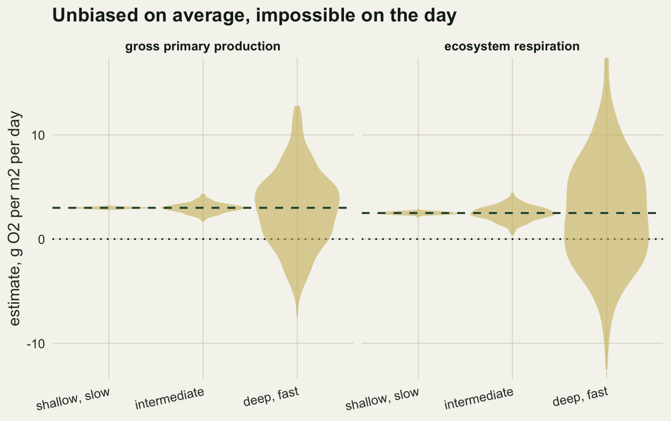
3 2.922 3.655 20.667 2.579 5.229 33.333 0.691The estimator is not biased. On the deep, fast reach the mean recovered production is 2.92 against a true 3.0, and the mean respiration is 2.58 against a true 2.5. Averaged over enough days it is right.
Individual days are another matter. The standard deviation of the daily production estimate rises from 0.09 on the shallow reach to 3.65 on the deep one, which is larger than the quantity being estimated. On that reach 20.7 per cent of days return negative gross primary production and 33.3 per cent return negative ecosystem respiration. Both are physically impossible: photosynthesis cannot consume oxygen and respiration cannot produce it. Nothing in the model is wrong, nothing in the fitting is wrong, and the sensor is behaving to specification.
The ratio inherits the damage. The median production to respiration ratio on the deep reach is 0.69 against a true 1.20, so a reach that is genuinely autotrophic is reported as heterotrophic on the typical day.
The coefficient you did not measure
Reaeration is rarely measured. It is usually taken from an empirical relationship with slope, velocity and depth, of the kind Raymond and colleagues assembled in 2012, and those relationships carry real scatter. Since gas exchange enters the same equation as the two fluxes being estimated, an error in it has to go somewhere.
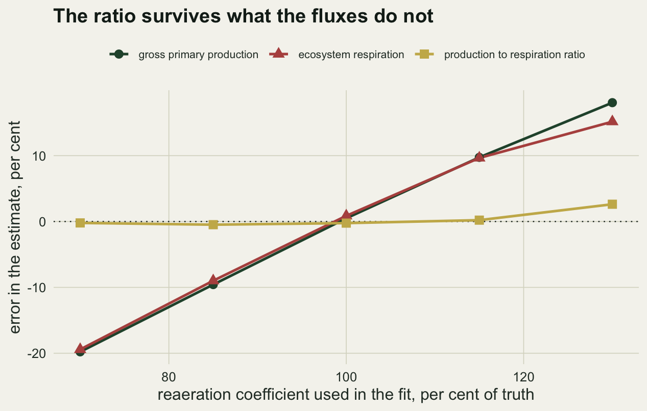
The sweep below fits the shallow reach, where the estimator is otherwise precise, with a reaeration coefficient set deliberately wrong by a fixed proportion.
k_factors <- c(0.70, 0.85, 1.00, 1.15, 1.30)
set.seed(5400)
sweep <- do.call(rbind, lapply(k_factors, function(f) {
  out <- t(replicate(80, {
    obs <- simulate_do(gpp_true, er_true, reaches$k_gas[1], reaches$depth[1],
                       noise = 0.15)
    fit_metab(obs, reaches$k_gas[1] * f, reaches$depth[1])
  }))
  data.frame(k_factor = f, gpp = mean(out[, 1]), er = mean(out[, 2]),
             pr = mean(out[, 1] / out[, 2]))
}))
sweep$gpp_error <- 100 * (sweep$gpp / gpp_true - 1)
sweep$er_error  <- 100 * (sweep$er / er_true - 1)
sweep$pr_error  <- 100 * (sweep$pr / (gpp_true / er_true) - 1)
round(sweep, 2)
k_factor gpp er pr gpp_error er_error pr_error
1 0.70 2.41 2.01 1.20 -19.79 -19.42 -0.21
2 0.85 2.71 2.28 1.19 -9.58 -8.99 -0.48
3 1.00 3.01 2.52 1.20 0.49 0.86 -0.24
4 1.15 3.29 2.74 1.20 9.74 9.65 0.21
5 1.30 3.54 2.88 1.23 18.05 15.16 2.62A reaeration coefficient set 30 per cent below the truth pulls gross primary production down by 19.8 per cent and ecosystem respiration down by 19.4 per cent. Both headline fluxes are wrong by roughly a fifth. The production to respiration ratio, computed from those same two wrong numbers, is off by 0.2 per cent.
That is not a coincidence. Gas exchange enters the mass balance as a single term applied to the whole day, so getting it wrong shifts the day’s oxygen budget up or down almost uniformly, and both fluxes absorb the shift in the same direction. What survives is their ratio, and what does not survive is either flux on its own.
What to report
Report the reach geometry next to the fluxes. Mean depth and the reaeration coefficient are not methods section trivia here, they are the two numbers that decide whether a daily estimate means anything, and a reader cannot judge a production figure without them.
Report the number of days that returned impossible values and what you did with them. Dropping negative estimates is not a neutral act: on the deep reach it discards 33 per cent of days, and those are the days on which the noise happened to push respiration low, so the surviving mean is biased upwards. Keeping them and averaging is defensible; deleting them silently is not.
If the argument rests on the balance between production and respiration rather than on either flux alone, say so, because the ratio is the quantity that tolerates an uncertain reaeration coefficient. If the argument rests on gross primary production as a number, the uncertainty in that number is dominated by the coefficient nobody measured, not by the sensor.
Honest limits
The failure on the deep reach is not equifinality. Fitting all three parameters at once from forty random starting points converges to a single solution every time, on both the shallow and the deep reach; the deep reach solution is simply the wrong one, precisely located. Appling and colleagues showed in 2018 that pooling many days does recover identifiability, but it does so by adding the assumption that reaeration is a smooth function of discharge, which is a modelling choice rather than a measurement.
Everything here is one photoperiod, one saturation concentration and one noise level. Real sensors drift, real saturation depends on temperature and pressure through the day, and real reaches are not well mixed boxes: groundwater arrives with its own oxygen concentration, and the water passing the sensor at dawn was somewhere else at midnight. The single station method assumes that upstream water looks like the water at the sensor, which is the assumption two station designs exist to remove.
The reaeration sweep treats the coefficient as a fixed multiple of the truth. Empirical scaling relationships also get the shape wrong, not just the level, so the error is not always a clean proportion. A tracer release measures the coefficient directly for the reach and the flow that was actually there, at the cost of a field day.
Finally, this post fits by least squares because it is transparent. Bayesian single station implementations such as the BASE approach of Grace and colleagues put priors on all three parameters, which prevents impossible values by construction. That is a genuine improvement in the output and a hidden change in the question: a posterior that cannot go below zero will report a small positive respiration on exactly the days when least squares reports an impossible one, and the underlying data is equally uninformative either way.
References
Odum HT 1956 Limnology and Oceanography 1(2):102-117 (10.4319/lo.1956.1.2.0102)
Raymond PA, Zappa CJ, Butman D, Bott TL, Potter J, Mulholland P, Laursen AE, McDowell WH, Newbold D 2012 Limnology and Oceanography Fluids and Environments 2(1):41-53 (10.1215/21573689-1597669)
Grace MR, Giling DP, Hladyz S, Caron V, Thompson RM, Mac Nally R 2015 Limnology and Oceanography Methods 13(3):103-114 (10.1002/lom3.10011)
Appling AP, Hall RO, Yackulic CB, Arroita M 2018 Journal of Geophysical Research Biogeosciences 123(2):624-645 (10.1002/2017JG004140)