library(ggplot2)
library(patchwork)

te_paper  <- "#f5f4ee"
te_ink    <- "#16241d"
te_body   <- "#2c3a31"
te_forest <- "#275139"
te_rust   <- "#b5534e"
te_gold   <- "#c9b458"
te_line   <- "#dad9ca"

theme_datasheet <- function() {
  theme_minimal(base_size = 12) +
    theme(plot.background  = element_rect(fill = te_paper, colour = NA),
          panel.background = element_rect(fill = te_paper, colour = NA),
          panel.grid.major = element_line(colour = te_line, linewidth = 0.3),
          panel.grid.minor = element_blank(),
          text             = element_text(colour = te_body),
          plot.title       = element_text(colour = te_ink, face = "bold"),
          plot.subtitle    = element_text(colour = te_body),
          axis.text        = element_text(colour = te_body))
}Chamber fluxes: linear or exponential fits
R
soil respiration
greenhouse gas flux
nonlinear regression
simulation
ecology tutorial
Closed chamber fluxes in R: the linear slope’s bias is a formula, while four syringe samples leave an exponential fit scattered and model choice adds error.
A grassland plot has a ring of steel collars pushed into the soil. Once a week a technician walks the plot with an opaque lid, seals it onto each collar for half an hour, and draws a syringe of headspace air at closure and after ten, twenty and thirty minutes. The vials go to a gas chromatograph. A neighbouring group on the same site uses a portable infrared analyser on a closed loop instead, and gets a concentration reading every minute from the same kind of lid. Both groups want one number per collar per week: the rate at which carbon dioxide leaves the soil surface.
The number is a slope, and the question is which slope. Sealing the lid changes the thing being measured. Gas accumulates in the headspace, the concentration difference that drives diffusion out of the soil shrinks, and the rise in concentration bends over. The flux the soil had before the lid went on is the slope at closure, not the average slope over the half hour. Hutchinson and Mosier wrote a flux equation for this bend in 1981, Kutzbach and colleagues showed in 2007 that linear regression on bending carbon dioxide records underestimates the flux even with short closures, and the choice between a straight line and a curve is still the first decision in a chamber data pipeline.
The site already has the tower above this instrument. Partitioning net flux into GPP and respiration splits eddy covariance net exchange into its gross components, and respiration appears there as a Lloyd and Taylor temperature curve, both generating the year of data and fitted to the night time fluxes; how the soil flux itself is measured never comes up. Stream metabolism from one oxygen logger has a gas exchange term too, but it is a reaeration coefficient between water and air, held at a value and then deliberately misset, not a feedback created by the measuring device. And checking a nonlinear model closes on the point that a fitted curve’s behaviour outside the data is a choice of form. Here the quantity wanted sits at the very edge of the data, at time zero, so the form matters even without extrapolating past the last sample.
The post separates what can be written down from what has to be simulated. The linear slope’s bias and error follow exactly from the curve and the sampling times, so they are derived and then checked against the simulation, not discovered by it. What has no formula is the exponential fit: how widely it scatters with four noisy samples, how often a standard fitting routine fails on it and which chambers those are, and what happens when the data are also used to choose between the line and the curve.
The headspace curve and the linear slope’s error
The truth used throughout is the single exponential headspace model. The soil emits an initial flux F0 into the headspace, and the rate of accumulation decays at a constant rate kappa as the headspace concentration approaches the soil gas concentration:
\[C(t) = C_0 + \frac{F_0}{\kappa}\left(1 - e^{-\kappa t}\right), \qquad C'(0) = F_0 .\]
Kappa is larger under a shallow lid than under a tall one, and in this model it is the only thing that makes the curve bend. The flux is expressed here as a concentration rate in ppm per minute, and multiplying by chamber volume over area and the gas density is the same for every estimator, so it is left out. The design constants below were fixed before any simulation was run.
f_true    <- 2          # initial flux into the headspace, ppm per minute
c_start   <- 420        # concentration at closure, ppm
kap_set   <- c(0.005, 0.02, 0.05)   # headspace feedback rate, per minute
close_set <- c(15, 30, 60)          # closure time, minutes
sd_set    <- c(1, 5)                # measurement noise, ppm
n_rep     <- 1000                   # simulated chambers per cell
kap_lo    <- 1e-5                   # bounds of the exponential fit
kap_hi    <- 0.2

sample_times <- function(protocol, closure) {
  if (protocol == "syringe") seq(0, closure, length.out = 4) else 0:closure
}
headspace <- function(tt, kap) c_start + (f_true / kap) * (1 - exp(-kap * tt))

# the linear slope and the quadratic slope at closure are weighted sums of the data
est_weights <- function(tt, estimator) {
  X <- if (estimator == "linear") cbind(1, tt) else cbind(1, tt, tt^2)
  solve(crossprod(X), t(X))[2, ]
}
closed_form <- function(tt, kap, noise_sd, estimator) {
  w <- est_weights(tt, estimator)
  bias <- sum(w * headspace(tt, kap)) / f_true - 1
  c(bias = bias, rmse = sqrt(bias^2 + noise_sd^2 * sum(w^2) / f_true^2))
}
lin_ratio_formula <- function(tt, kap) {
  tc <- tt - mean(tt)
  -sum(tc * exp(-kap * tt)) / (kap * sum(tc^2))
}
formula_gap <- max(abs(unlist(lapply(kap_set, function(k) lapply(close_set, function(cl)
  vapply(c("syringe", "analyser"), function(p) {
    tt <- sample_times(p, cl)
    (lin_ratio_formula(tt, k) - 1) - closed_form(tt, k, 1, "linear")[["bias"]]
  }, 0))))))

tt_syr <- sample_times("syringe", 30); tt_ana <- sample_times("analyser", 30)
cf_syr5 <- closed_form(tt_syr, 0.02, 5, "linear")
cf_ana1 <- closed_form(tt_ana, 0.02, 1, "linear")
cf_ana5 <- closed_form(tt_ana, 0.02, 5, "linear")
cf_q_syr5 <- closed_form(tt_syr, 0.02, 5, "quadratic")
cf_q_ana1 <- closed_form(tt_ana, 0.02, 1, "quadratic")
rise_30 <- headspace(30, 0.02) - c_start
The ordinary least squares slope is a fixed weighted sum of the observations, with weights proportional to each sampling time’s distance from the mean time. Its expectation is therefore the same weighted sum of the true curve, and the constant C0 drops out because the weights sum to zero. Writing that out gives the ratio of the expected slope to the true initial flux:
\[\frac{E(\hat b)}{F_0} = -\frac{\sum_i (t_i - \bar t)\, e^{-\kappa t_i}}{\kappa \sum_i (t_i - \bar t)^2} ,\]
and the variance of the slope is the noise variance divided by the sum of squares of the times, exactly as for any regression. Neither involves the flux itself except as a scale: the relative bias depends only on kappa and the sampling times, and for equally spaced times it depends only on the product of kappa and the closure time and on the number of samples. The formula and the direct matrix computation in the chunk agree to 4.88e-15.
At kappa 0.02 per minute and a 30 minute closure, the headspace rises by 45.1 ppm against the 60 ppm a constant flux would give. The linear slope through the four syringe samples then has a relative bias of -0.249 and, with 5 ppm of noise per sample, a relative root mean squared error of 0.273. The analyser’s 31 readings at 1 ppm of noise give a bias of -0.252 and an error of 0.252. More and better data barely change the error, because nearly all of it is bias, and bias does not average away. The same algebra applies to the slope at closure from a quadratic fit, which is also a weighted sum of the observations: its bias with the four syringe samples is only -0.025, but its error with 5 ppm of noise is 0.392, because a curvature estimated from four points is noisy.
set.seed(4107)
ex_ana <- data.frame(tt = tt_ana, conc = headspace(tt_ana, 0.02) + rnorm(length(tt_ana), 0, 1))
ex_syr <- data.frame(tt = tt_syr, conc = headspace(tt_syr, 0.02) + rnorm(length(tt_syr), 0, 1))
ex_fit <- lm(conc ~ tt, data = ex_ana)
curve_df <- data.frame(tt = seq(0, 30, by = 0.25))
curve_df$truth   <- headspace(curve_df$tt, 0.02)
curve_df$tangent <- c_start + f_true * curve_df$tt
curve_df$linfit  <- predict(ex_fit, newdata = curve_df)
long_curve <- rbind(
  data.frame(tt = curve_df$tt, conc = curve_df$truth,   what = "true headspace curve"),
  data.frame(tt = curve_df$tt, conc = curve_df$tangent, what = "initial flux (tangent)"),
  data.frame(tt = curve_df$tt, conc = curve_df$linfit,  what = "linear fit to analyser"))
p_curve <- ggplot() +
  geom_line(data = long_curve, aes(tt, conc, colour = what, linetype = what), linewidth = 0.9) +
  geom_point(data = ex_ana, aes(tt, conc), colour = te_ink, size = 1, alpha = 0.6) +
  geom_point(data = ex_syr, aes(tt, conc), colour = te_rust, size = 3, shape = 17) +
  scale_colour_manual(values = c("true headspace curve" = te_ink,
                                 "initial flux (tangent)" = te_forest,
                                 "linear fit to analyser" = te_gold), name = NULL) +
  scale_linetype_manual(values = c("true headspace curve" = "solid",
                                   "initial flux (tangent)" = "dashed",
                                   "linear fit to analyser" = "solid"), name = NULL) +
  labs(x = "minutes since closure", y = "CO2 in headspace (ppm)", title = "One chamber") +
  theme_datasheet() + theme(legend.position = "bottom", legend.direction = "vertical")

kt_grid <- seq(0.01, 3.5, length.out = 120)
bias_curve <- rbind(
  data.frame(kt = kt_grid, protocol = "4 syringe samples",
             bias = vapply(kt_grid, function(v) lin_ratio_formula(seq(0, 30, length.out = 4), v / 30) - 1, 0)),
  data.frame(kt = kt_grid, protocol = "analyser, 1 per minute",
             bias = vapply(kt_grid, function(v) lin_ratio_formula(0:30, v / 30) - 1, 0)))
p_bias <- ggplot(bias_curve, aes(kt, bias, colour = protocol)) +
  geom_hline(yintercept = 0, colour = te_line) +
  geom_line(linewidth = 0.9) +
  scale_colour_manual(values = c("4 syringe samples" = te_rust, "analyser, 1 per minute" = te_forest), name = NULL) +
  labs(x = "kappa x closure time", y = "relative bias of linear slope", title = "Bias from the formula") +
  theme_datasheet() + theme(legend.position = "bottom", legend.direction = "vertical")
p_curve + p_bias + plot_annotation(theme = theme_datasheet())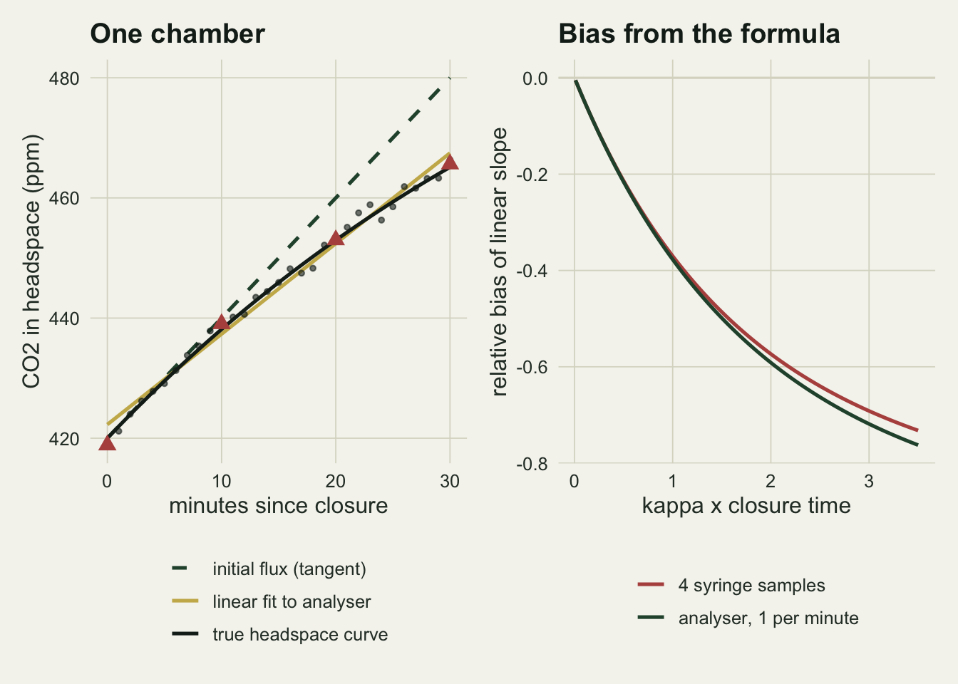
A grid of simulated chambers
The simulation crosses the three kappa values, the two protocols, the two noise levels and the three closure times, giving 36 cells of 1000 chambers each. The four syringe samples are always spread evenly over the closure, and the analyser reads once a minute from closure to the end. Every chamber gets three estimates of the initial flux.
The linear and quadratic estimates are plain least squares. The exponential estimate is bounded least squares on the headspace model, with kappa kept between 0.00001 and 0.2 per minute. It is computed by profiling: for any fixed kappa the model is linear in C0 and F0, so the residual sum of squares is available in closed form, and the fit reduces to a one dimensional minimisation over kappa, done here on a grid of 300 values followed by a local search. That cannot fail to converge, which matters below. When the minimum sits at the lower bound of kappa the model has collapsed into a straight line, and the exponential estimate is, to within rounding, the linear slope.
kgrid_make <- function(upper) exp(seq(log(kap_lo), log(upper), length.out = 300))

# for a fixed kappa the exponential model is linear in C0 and F0
rss_at <- function(tt, Y, kap) {
  x  <- (1 - exp(-kap * tt)) / kap
  xc <- x - mean(x); sxx <- sum(xc^2)
  Yc <- Y - rep(colMeans(Y), each = length(tt))
  slope <- colSums(xc * Yc) / sxx
  list(rss = colSums(Yc^2) - slope^2 * sxx, flux = slope)
}

fit_chambers <- function(tt, Y, upper = kap_hi) {
  n_obs <- length(tt); n_ch <- ncol(Y); kgrid <- kgrid_make(upper)
  rss_mat <- vapply(kgrid, function(k) rss_at(tt, Y, k)$rss, numeric(n_ch))
  rss_mat <- matrix(rss_mat, nrow = n_ch)
  best <- max.col(-rss_mat, ties.method = "first")
  kap_hat <- flux_exp <- rss_exp <- numeric(n_ch)
  for (r in seq_len(n_ch)) {
    brk <- log(kgrid[c(max(best[r] - 1, 1), min(best[r] + 1, length(kgrid)))])
    y_r <- Y[, r, drop = FALSE]
    opt <- optimize(function(lk) rss_at(tt, y_r, exp(lk))$rss, brk)
    kap_hat[r] <- exp(opt$minimum)
    z <- rss_at(tt, y_r, kap_hat[r])
    flux_exp[r] <- z$flux; rss_exp[r] <- z$rss
  }
  X1 <- cbind(1, tt); b1 <- solve(crossprod(X1), crossprod(X1, Y))
  rss_lin <- colSums((Y - X1 %*% b1)^2)
  X2 <- cbind(1, tt, tt^2); b2 <- solve(crossprod(X2), crossprod(X2, Y))
  rss_q <- colSums((Y - X2 %*% b2)^2)
  se_q2 <- sqrt(rss_q / (n_obs - 3) * solve(crossprod(X2))[3, 3])
  data.frame(linear = b1[2, ], quadratic = b2[2, ], exponential = flux_exp,
             kap_hat = kap_hat,
             at_lower = kap_hat < kgrid[2], at_upper = kap_hat > kgrid[length(kgrid) - 1],
             aic_lin = n_obs * log(rss_lin / n_obs) + 2 * 3,
             aic_exp = n_obs * log(rss_exp / n_obs) + 2 * 4,
             p_curv  = 2 * pt(-abs(b2[3, ] / se_q2), n_obs - 3),
             curv    = b2[3, ])
}
Two selection rules are applied to the same chambers. The AIC rule takes the exponential estimate when its AIC is lower than the linear model’s, counting the residual variance as a parameter in both. The curvature rule fits the quadratic and takes the exponential estimate only when the squared term is negative and significant at the 5 per cent level, and the linear slope otherwise. The AIC rule is not applied to the syringe protocol, for a reason given in the rules section.
cells <- expand.grid(kap = kap_set, protocol = c("syringe", "analyser"),
                     noise_sd = sd_set, closure = close_set, stringsAsFactors = FALSE)
set.seed(20260904)
sims <- lapply(seq_len(nrow(cells)), function(i) {
  cl <- cells[i, ]; tt <- sample_times(cl$protocol, cl$closure)
  Y <- headspace(tt, cl$kap) + matrix(rnorm(length(tt) * n_rep, 0, cl$noise_sd), length(tt))
  out <- fit_chambers(tt, Y)
  # AIC is not applied with 4 points and 4 parameters
  out$aic_rule  <- if (cl$protocol == "syringe") NA_real_ else
    ifelse(out$aic_exp < out$aic_lin, out$exponential, out$linear)
  out$curv_rule <- ifelse(out$p_curv < 0.05 & out$curv < 0, out$exponential, out$linear)
  data.frame(cl, out, row.names = NULL)
})

rel_rmse <- function(v) sqrt(mean((v / f_true - 1)^2))
summ <- do.call(rbind, lapply(sims, function(d) {
  tt <- sample_times(d$protocol[1], d$closure[1])
  cf_l <- closed_form(tt, d$kap[1], d$noise_sd[1], "linear")
  cf_q <- closed_form(tt, d$kap[1], d$noise_sd[1], "quadratic")
  data.frame(d[1, c("kap", "protocol", "noise_sd", "closure")], row.names = NULL,
    lin_bias_sim = mean(d$linear) / f_true - 1, lin_bias_cf = cf_l[["bias"]],
    lin_se_cf = sqrt(cf_l[["rmse"]]^2 - cf_l[["bias"]]^2) / sqrt(n_rep),
    lin_rmse_sim = rel_rmse(d$linear), lin_rmse_cf = cf_l[["rmse"]],
    quad_rmse_sim = rel_rmse(d$quadratic), quad_rmse_cf = cf_q[["rmse"]],
    exp_rmse = rel_rmse(d$exponential),
    exp_q05 = unname(quantile(d$exponential / f_true, 0.05)),
    exp_q50 = median(d$exponential / f_true),
    exp_q95 = unname(quantile(d$exponential / f_true, 0.95)),
    exp_lower = mean(d$at_lower), exp_upper = mean(d$at_upper),
    aic_rmse = if (is.na(d$aic_rule[1])) NA_real_ else rel_rmse(d$aic_rule),
    aic_pick = if (is.na(d$aic_rule[1])) NA_real_ else mean(d$aic_exp < d$aic_lin),
    curv_rmse = rel_rmse(d$curv_rule),
    curv_pick = mean(d$p_curv < 0.05 & d$curv < 0))
}))
row.names(summ) <- NULL
z_gap_bias <- max(abs(summ$lin_bias_sim - summ$lin_bias_cf) / summ$lin_se_cf)
gap_rmse_lin  <- max(abs(summ$lin_rmse_sim - summ$lin_rmse_cf))
gap_rmse_quad <- max(abs(summ$quad_rmse_sim - summ$quad_rmse_cf) / summ$quad_rmse_cf)
pick_cell <- function(k, p, s, cl) summ[summ$kap == k & summ$protocol == p & summ$noise_sd == s & summ$closure == cl, ]
get_sim   <- function(k, p, s, cl) sims[[which(cells$kap == k & cells$protocol == p & cells$noise_sd == s & cells$closure == cl)]]
c_syr5 <- pick_cell(0.02, "syringe", 5, 30)
c_syr1 <- pick_cell(0.02, "syringe", 1, 30)
c_ana5 <- pick_cell(0.02, "analyser", 5, 30)
c_ana1 <- pick_cell(0.02, "analyser", 1, 30)
c_syr5_k05 <- pick_cell(0.05, "syringe", 5, 30)
exp_beats_lin <- sum(summ$exp_rmse < summ$lin_rmse_cf)
quad_best <- sum(summ$quad_rmse_cf < pmin(summ$lin_rmse_cf, summ$exp_rmse))
lin_best  <- sum(summ$lin_rmse_cf < pmin(summ$quad_rmse_cf, summ$exp_rmse))
n_cells <- nrow(summ)
The simulation is a check on the formula before it is anything else. Across all 36 cells the simulated mean of the linear slope sits within 1.5 Monte Carlo standard errors of the formula’s bias at worst, the simulated linear error differs from its closed form by at most 0.010, and the quadratic’s simulated error is within 4 per cent of its own closed form. Nothing about the two regression slopes needed simulating. What follows is about the estimate that does.
Over the whole grid the exponential fit has a lower error than the straight line in 21 of the 36 cells, the straight line is best of the three in 13, and the quadratic slope at closure is best in 13. There is no single winner, and the ranking changes along the closure time and protocol axes at a fixed kappa, so the same soil can favour a different estimator under a different sampling plan.
Four syringe samples and the exponential fit
With the analyser at 1 ppm of noise, kappa 0.02 and a 30 minute closure, the exponential estimate does what the textbook promises. Its median is 1.000 of the true flux, 90 per cent of chambers fall between 0.93 and 1.08, and its relative error is 0.049 against the linear slope’s 0.252.
d_syr5 <- get_sim(0.02, "syringe", 5, 30)
syr5_mean <- mean(d_syr5$exponential) / f_true
lower_upcurve  <- mean(d_syr5$curv[d_syr5$at_lower] > 0)
lower_is_upcurve <- mean(d_syr5$at_lower == (d_syr5$curv > 0))
upcurve_share  <- mean(d_syr5$curv > 0)
lower_lin_gap  <- max(abs(d_syr5$exponential - d_syr5$linear)[d_syr5$at_lower]) / f_true
mean_lower     <- mean(d_syr5$exponential[d_syr5$at_lower]) / f_true
mean_rest      <- mean(d_syr5$exponential[!d_syr5$at_lower]) / f_true
Take the same soil and lid with four syringe samples at 5 ppm of noise and the picture changes. The median is still 1.004, so half the chambers fall on each side of the truth, but the mean is 1.130, and the central 90 per cent of estimates runs from 0.63 to 2.01 times the truth. The relative error is 0.483, against 0.273 for the biased straight line and 0.392 for the quadratic. The spread is lopsided, with a long upper tail, which is the positively skewed distribution Venterea, Spokas and Baker described for nonlinear flux schemes.
In a sizeable share of chambers the fit returns a straight line. In 28.2 per cent of these chambers the best kappa is at the lower bound, so the reported exponential flux is in effect the linear slope with its full bias; in 0.3 per cent it is at the upper bound. The estimate is a mixture. The lower bound catches the chambers where noise has made the record curve upwards: 100 per cent of them have a positive squared term in the quadratic fit, 28.2 per cent of all chambers curve upwards, and the two groups coincide in 100.0 per cent of chambers. A saturating curve cannot bend that way, so the bounded fit returns the straight line (the two slopes differ by at most 1.6e-04 times the true flux there) and averages 0.75 of the truth. In the rest, noise and curvature are fitted together, the slope at closure can swing well above the truth, and the mean is 1.28. At kappa 0.05 with the same samples the range widens to 0.44 to 2.55 and the error to 0.700.
spread_df <- do.call(rbind, lapply(c("syringe", "analyser"), function(p) {
  d <- get_sim(0.02, p, 5, 30)
  lab <- if (p == "syringe") "4 syringe samples, sd 5 ppm" else "analyser every minute, sd 5 ppm"
  rbind(data.frame(ratio = d$linear / f_true, estimator = "linear", panel = lab),
        data.frame(ratio = d$quadratic / f_true, estimator = "quadratic", panel = lab),
        data.frame(ratio = d$exponential / f_true, estimator = "exponential", panel = lab))
}))
spread_df$panel <- factor(spread_df$panel,
                          levels = c("4 syringe samples, sd 5 ppm", "analyser every minute, sd 5 ppm"))
ggplot(spread_df, aes(ratio, colour = estimator)) +
  geom_vline(xintercept = 1, colour = te_ink, linetype = "dashed") +
  geom_density(linewidth = 0.9, adjust = 0.8) +
  coord_cartesian(xlim = c(-0.25, 3)) +
  scale_colour_manual(values = c(linear = te_gold, quadratic = te_forest, exponential = te_rust), name = NULL) +
  facet_wrap(~ panel, ncol = 1, scales = "free_y") +
  labs(x = "estimated flux / true initial flux", y = "density") +
  theme_datasheet() + theme(legend.position = "bottom")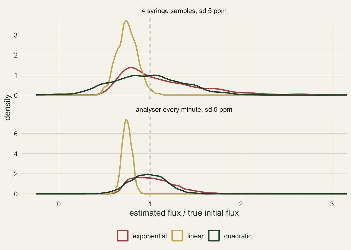
Failed fits are not a random subset
The profile fit above never fails. A common route in R is nls() with bounds, started from the linear fit and a guess for kappa, and that does fail on some data sets. The next chunk fits fresh chambers at kappa 0.02, 5 ppm of noise and a 30 minute closure with nls(algorithm = "port") under the same bounds, and compares every chamber with the profile fit of the same data.
nls_check <- function(protocol, n_ch = 1000) {
  tt <- sample_times(protocol, 30)
  Y <- headspace(tt, 0.02) + matrix(rnorm(length(tt) * n_ch, 0, 5), length(tt))
  prof <- fit_chambers(tt, Y)
  flux_nls <- rep(NA_real_, n_ch)
  for (r in seq_len(n_ch)) {
    y <- Y[, r]; st <- coef(lm(y ~ tt))
    fit <- tryCatch(nls(y ~ a + (fl / kp) * (1 - exp(-kp * tt)),
                        start = list(a = st[[1]], fl = st[[2]], kp = 0.01),
                        algorithm = "port", lower = c(-Inf, -Inf, kap_lo), upper = c(Inf, Inf, kap_hi)),
                    error = function(e) NULL)
    if (!is.null(fit)) flux_nls[r] <- coef(fit)[["fl"]]
  }
  ok <- !is.na(flux_nls)
  data.frame(protocol = protocol, fail = mean(!ok), fail_se = sqrt(mean(!ok) * mean(ok) / n_ch),
             agree99 = unname(quantile(abs(flux_nls[ok] - prof$exponential[ok]) / f_true, 0.99)),
             lower_all = mean(prof$at_lower), lower_fail = mean(prof$at_lower[!ok]),
             ratio_fail = mean(prof$exponential[!ok]) / f_true,
             ratio_ok = mean(prof$exponential[ok]) / f_true,
             ratio_all = mean(prof$exponential) / f_true, n_fail = sum(!ok))
}
set.seed(918)
nls_tab <- rbind(nls_check("syringe"), nls_check("analyser"))
nls_s <- nls_tab[1, ]; nls_a <- nls_tab[2, ]
nls() stops with an error on 3.0 per cent of the syringe chambers (Monte Carlo standard error 0.5) and 3.2 per cent of the analyser chambers (0.6). Where it converges it finds the same answer as the profile fit: 99 per cent of the converged chambers agree to within 2.9e-05 times the true flux with syringes and 2.0e-05 with the analyser. So the failures belong to the algorithm and its starting values, not to the model.
They are not random, though. Among the syringe chambers where nls() failed, the profile fit put kappa on its lower bound 57 per cent of the time, against 27 per cent overall; for the analyser the two shares are 75 and 11 per cent. The routine fails most often where the record shows no downward curvature, and those chambers have low exponential estimates: a mean of 0.79 of the true flux among the failures, against 1.14 among the successes. Dropping failed chambers from the syringe data set moves the mean exponential estimate from 1.132 to 1.143 of the truth. With these failure rates that shift is small, but its direction is fixed, and a pipeline that silently discards non-converging chambers is removing the low ones.
Choosing the model from the same data
The practical answer to the spread is usually a rule: fit both and keep the curve only when the data support it. Kutzbach and colleagues fitted both models and examined the residuals; Pedersen, Petersen and Schelde built the HMR procedure, which sorts each chamber record into a nonlinear case fitted with the exponential headspace model, a linear case, or no detectable flux, and is distributed as an R package. HMR makes that decision with its own criteria and those are not reproduced here. The two rules below are simpler stand ins of the same kind.
The AIC rule cannot be used honestly on four syringe samples. The exponential model has three parameters for the mean and one for the noise, which is as many as there are observations: the small sample correction to AIC divides by the number of observations minus the number of parameters minus one, which is negative here, and the plain AIC would be comparing a fit with one residual degree of freedom against a fit with two. The curvature rule can be computed with four samples, but its t test has a single degree of freedom and needs a t statistic above 12.7, so it takes the curve in at most 40 per cent of chambers in any syringe cell, and in 4.9 per cent at kappa 0.02, 5 ppm of noise and a 30 minute closure, where it nearly always reports the linear slope.
d_sel <- get_sim(0.02, "analyser", 5, 30)
err2 <- function(v) (v / f_true - 1)^2
diff_exp <- err2(d_sel$aic_rule) - err2(d_sel$exponential)
diff_lin <- err2(d_sel$aic_rule) - err2(d_sel$linear)
mse_gap_exp <- mean(diff_exp); mse_gap_exp_se <- sd(diff_exp) / sqrt(n_rep)
mse_gap_lin <- mean(diff_lin); mse_gap_lin_se <- sd(diff_lin) / sqrt(n_rep)
picked <- d_sel$aic_exp < d_sel$aic_lin
share_picked <- mean(picked)
mean_exp_picked    <- mean(d_sel$exponential[picked]) / f_true
mean_exp_notpicked <- mean(d_sel$exponential[!picked]) / f_true
mean_lin_notpicked <- mean(d_sel$linear[!picked]) / f_true
mean_rule <- mean(d_sel$aic_rule) / f_true

ana_cells <- summ[summ$protocol == "analyser", ]
n_ana <- nrow(ana_cells)
aic_worse_both <- sum(ana_cells$aic_rmse > pmax(ana_cells$lin_rmse_cf, ana_cells$exp_rmse))
aic_between    <- sum(ana_cells$aic_rmse <= pmax(ana_cells$lin_rmse_cf, ana_cells$exp_rmse) &
                      ana_cells$aic_rmse > pmin(ana_cells$lin_rmse_cf, ana_cells$exp_rmse))
aic_worse_exp  <- sum(ana_cells$aic_rmse > ana_cells$exp_rmse)
aic_all_exp <- sum(ana_cells$aic_pick == 1)
aic_best <- sum(ana_cells$aic_rmse < pmin(ana_cells$lin_rmse_cf, ana_cells$exp_rmse))
curv_worse_both <- sum(summ$curv_rmse > pmax(summ$lin_rmse_cf, summ$exp_rmse))
At kappa 0.02, 5 ppm of noise and a 30 minute analyser record, the AIC rule takes the curve in 45 per cent of chambers. Its relative error is 0.278, higher than the exponential fit’s 0.239 and also higher than the linear slope’s 0.257. Paired over the same chambers, the rule’s mean squared error exceeds the exponential fit’s by 0.0204 (standard error 0.0009) and the straight line’s by 0.0107 (standard error 0.0031), so in this cell the rule is worse than either model used on its own. The curvature rule does no better here, at 0.294.
The mechanism is the one familiar from any pretest. The true curvature is identical in every chamber of this cell, so what separates the chambers where AIC picks the curve from those where it does not is the noise, and the curve is picked when the noise has made the record look more bent. In the chambers where AIC took the exponential fit its estimate averaged 1.24 of the true flux. In the rest the rule reported the linear slope, which averaged 0.75, where the exponential fit would have given 0.87. Averaged together the rule’s mean is 0.972, close to the truth, but that mean is an average of two groups that are wrong in opposite directions, and the squared error does not cancel the way the mean does.
pick_df <- data.frame(linear = d_sel$linear / f_true, exponential = d_sel$exponential / f_true,
                      choice = ifelse(picked, "AIC takes exponential", "AIC takes linear"))
ggplot(pick_df, aes(linear, exponential, colour = choice)) +
  geom_hline(yintercept = 1, colour = te_ink, linetype = "dashed") +
  geom_abline(slope = 1, intercept = 0, colour = te_body, linetype = "dotted") +
  geom_point(size = 1.1, alpha = 0.6) +
  scale_colour_manual(values = c("AIC takes exponential" = te_rust, "AIC takes linear" = te_forest), name = NULL) +
  labs(x = "linear estimate / true flux", y = "exponential estimate / true flux") +
  theme_datasheet() + theme(legend.position = "bottom")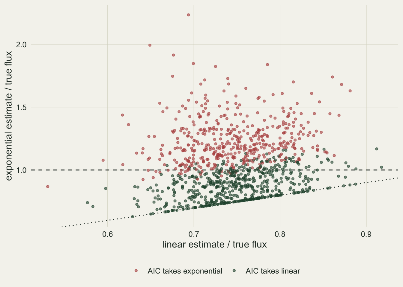
That cell is the exception, not the typical case. Across the 18 analyser cells the AIC rule is worse than both single models in 1, lies between them in 10, and is worse than always fitting the exponential in 6. The curvature rule is worse than both in 3 of all 36 cells. In the remaining 7 analyser cells, the long or low-noise records where the bend is resolved, AIC picks the curve in every chamber and the rule is the exponential fit. It beats both of the models it chooses between in 0 of the 18 cells. What it buys is protection in the cells where the exponential fit is poor and the straight line better; what it costs is error in the cells where the exponential fit alone would have done better.
rules_df <- do.call(rbind, lapply(seq_len(nrow(summ)), function(i) {
  s <- summ[i, ]
  data.frame(s[c("kap", "protocol", "noise_sd", "closure")], row.names = NULL,
    estimator = c("linear", "quadratic", "exponential", "AIC rule", "curvature rule"),
    rmse = c(s$lin_rmse_cf, s$quad_rmse_cf, s$exp_rmse, s$aic_rmse, s$curv_rmse))
}))
rules_df <- rules_df[rules_df$noise_sd == 5 & !is.na(rules_df$rmse), ]
rules_df$kap_lab <- factor(paste("kappa", rules_df$kap), levels = paste("kappa", kap_set))
rules_df$protocol <- factor(ifelse(rules_df$protocol == "syringe", "4 syringe samples", "analyser every minute"),
                            levels = c("4 syringe samples", "analyser every minute"))
ggplot(rules_df, aes(closure, rmse, colour = estimator, linetype = estimator)) +
  geom_line(linewidth = 0.8) + geom_point(size = 1.6) +
  scale_y_log10() + scale_x_continuous(breaks = close_set) +
  scale_colour_manual(values = c(linear = te_gold, quadratic = te_forest, exponential = te_rust,
                                 "AIC rule" = te_ink, "curvature rule" = "#7c8b80"), name = NULL) +
  scale_linetype_manual(values = c(linear = "solid", quadratic = "solid", exponential = "solid",
                                   "AIC rule" = "dashed", "curvature rule" = "dotted"), name = NULL) +
  facet_grid(protocol ~ kap_lab) +
  labs(x = "closure time (minutes)", y = "relative RMSE of the flux (log scale)") +
  theme_datasheet() + theme(legend.position = "bottom")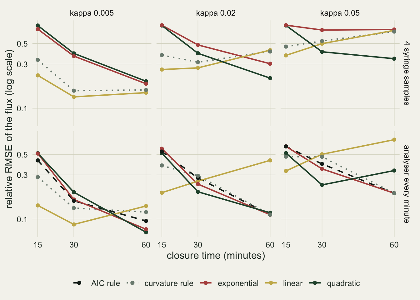
One design constant could be driving the syringe tail: the upper bound of 0.2 per minute on kappa. The chunk below refits one set of syringe chambers with the bound raised to 1.
set.seed(77)
Y_up <- headspace(tt_syr, 0.02) + matrix(rnorm(4 * n_rep, 0, 5), 4)
up_02 <- fit_chambers(tt_syr, Y_up, upper = kap_hi)
up_1  <- fit_chambers(tt_syr, Y_up, upper = 1)
up_rmse_02 <- rel_rmse(up_02$exponential); up_rmse_1 <- rel_rmse(up_1$exponential)
up_hits_02 <- mean(up_02$at_upper); up_hits_1 <- mean(up_1$at_upper)
The relative error is 0.444 with the bound at 0.2 and 0.449 with it at 1, and the share of fits at the upper bound is 0.1 and 0.0 per cent. The spread of the four sample exponential fit comes from the data, not from where the bound was put. These chambers are a fresh draw, and the grid cell with the same settings gave 0.483: the root mean squared error of a long tailed estimate moves noticeably between runs of 1000 chambers, which is why the quantiles are the more stable summary.
What to report
Report the sampling protocol with the flux: closure time, number and timing of samples, and the analytical noise of the instrument, because these set the error of whichever estimator is used. A flux without them cannot be compared with another study’s flux, even from the same soil.
If the linear slope was used, report closure time and, if it is available, a typical curvature or kappa from records where it could be estimated, and give the implied bias from the formula above. The bias is not a vague caveat; it is a number that follows from kappa and the sampling times, and at kappa 0.05 with a 60 minute closure it is -0.721 for the analyser.
If the exponential fit was used with few samples, report the share of chambers where the curvature parameter ended on a bound and the number of fits that did not converge, and say what was done with them. Discarding non-converged chambers removes records that show no downward curvature, whose estimates are low, and so moves the mean upwards.
If a selection rule chose between models, name the rule, give the share of chambers assigned to each model, and treat the reported flux as coming from the rule, not from whichever model was selected in a particular chamber. Its error is that of the mixture, which can be larger than the error of either model used consistently.
Honest limits
The truth here is the single exponential model with a constant kappa, and it is also the model being fitted, which is the best case for the exponential estimate. Real headspace curves depart from it: soil gas diffuses from a profile rather than from one well mixed reservoir, and Kutzbach and colleagues found many records whose curvature did not match the theoretical shape, which they put down to turbulence and pressure disturbances when the lid went on. Under a diffusion profile truth the exponential fit can carry a bias of its own, and the comparison with the straight line could shift; that case was not run. No leaks, pressure pulses, temperature change inside the lid or plant uptake were simulated.
Noise is independent and normal with a constant standard deviation. Syringe sampling adds handling error that grows with concentration, and analyser records are autocorrelated over a few readings, which makes 31 readings worth fewer independent observations than the number suggests.
The flux is always positive and well above the noise. Nitrous oxide and methane fluxes near detection limits, where the sign of the slope is uncertain and HMR’s no flux category matters, were not simulated, and the relative error used throughout is not meaningful when the true flux is close to zero.
The two selection rules are simplified stand ins. HMR’s own decisions, and the minimum detectable flux thresholds used in many pipelines, are different rules with their own error; the general point that a data driven choice adds its own error carries over, but the numbers do not. The failure rate of nls() depends on the starting values and algorithm, and the rate measured here belongs to the start used in the chunk, not to nonlinear least squares in general.
References
Hutchinson GL, Mosier AR 1981 Soil Science Society of America Journal 45(2):311-316 (10.2136/sssaj1981.03615995004500020017x)
Kutzbach L, Schneider J, Sachs T, Giebels M, Nykanen H, Shurpali NJ, Martikainen PJ, Alm J, Wilmking M 2007 Biogeosciences 4(6):1005-1025 (10.5194/bg-4-1005-2007)
Venterea RT, Spokas KA, Baker JM 2009 Soil Science Society of America Journal 73(4):1087-1093 (10.2136/sssaj2008.0307)
Pedersen AR, Petersen SO, Schelde K 2010 European Journal of Soil Science 61(6):888-902 (10.1111/j.1365-2389.2010.01291.x)