library(ggplot2)
library(patchwork)

te_paper  <- "#f5f4ee"
te_ink    <- "#16241d"
te_body   <- "#2c3a31"
te_forest <- "#275139"
te_rust   <- "#b5534e"
te_gold   <- "#c9b458"
te_line   <- "#dad9ca"

theme_datasheet <- function() {
  theme_minimal(base_size = 12) +
    theme(plot.background  = element_rect(fill = te_paper, colour = NA),
          panel.background = element_rect(fill = te_paper, colour = NA),
          panel.grid.major = element_line(colour = te_line, linewidth = 0.3),
          panel.grid.minor = element_blank(),
          text             = element_text(colour = te_body),
          plot.title       = element_text(colour = te_ink, face = "bold"),
          plot.subtitle    = element_text(colour = te_body),
          axis.text        = element_text(colour = te_body),
          strip.text       = element_text(colour = te_ink))
}Pretesting variances before a t test
R
hypothesis testing
simulation
statistics
ecology tutorial
Checking equal variances before choosing the pooled t test is a test with its own error rate. Measured in R: passing the pretest makes the pooled t less safe.
Ten restored ponds and thirty long established reference ponds, one net sweep survey in each, and the response is the log density of dragonfly larvae. The restored ponds are younger and less settled, so they vary more from one to the next. The analysis plan most people would write down is short. Check whether the two groups have equal variances; if the check passes, run the ordinary two sample t test with a pooled variance; if it fails, switch to the Welch test. Some plans do the same with a normality check and a Wilcoxon test as the fallback.
The plan reads like caution. It is also a statistical procedure in its own right, made of two tests in sequence, and its error rate is not the error rate of either test on its own. Nobody computes that rate, because the output at the end is a single p value from a single named test, and the pretest that chose it has vanished from the report.
What a rank test actually tests already shows that the pooled t test fails under unequal spread and the Welch test does not: with fifteen observations in the more variable group and forty five in the tighter one, it reports the unconditional rejection rates of the three tests side by side. It never runs the two stage rule and never asks what happens to the pooled test in the samples where a variance check came back clean. That is the question here: the rule most people actually follow, and whether passing the check makes the pooled test safe.
Two other posts carry half of the argument already. Testing for no effect is about the gap between failing to detect a difference and showing that there is none; a variance pretest that does not reject is that same gap, applied to two standard deviations instead of two means. Checking a penalised regression runs a coverage experiment on intervals computed after the lasso has chosen the variables, and finds that intervals which look valid are not, because the data that did the choosing are reused for the inference. The two stage t test is the smallest example of that problem that exists: one binary choice, one test, and a closed form for every piece except the combination.
Four tests written as matrix arithmetic
Every test in this post is computed by hand on whole matrices of simulated data, one row per replicate dataset, so that tens of thousands of datasets cost a fraction of a second. That makes it necessary to show that the hand versions are the tests they claim to be.
The pooled t test uses the variance pooled over both groups on n1 + n2 - 2 degrees of freedom. The Welch test uses the separate variances and the Welch-Satterthwaite degrees of freedom, as t.test does by default. Two variance pretests are carried. The first is the F test on the ratio of the sample variances, two sided, which is what var.test computes. The second is the Brown-Forsythe version of Levene’s test: take the absolute deviation of every observation from its own group median and run a one way analysis of variance on those deviations. Levene proposed deviations from the group mean; Brown and Forsythe (1974) replaced the mean by the median, which keeps the test’s level when the data are skewed, and it is the default in the most widely used R implementation. With two groups the analysis of variance F statistic is the square of a pooled t statistic on the deviations, which is how it is computed below.
row_var <- function(m) {
  mu <- rowMeans(m)
  rowSums((m - mu)^2) / (ncol(m) - 1)
}

row_tests <- function(x1, x2, sd1 = NA, sd2 = NA) {
  n1 <- ncol(x1)
  n2 <- ncol(x2)
  m1 <- rowMeans(x1)
  m2 <- rowMeans(x2)
  v1 <- row_var(x1)
  v2 <- row_var(x2)
  df_pool <- n1 + n2 - 2
  sp2     <- ((n1 - 1) * v1 + (n2 - 1) * v2) / df_pool
  t_pool  <- (m1 - m2) / sqrt(sp2 * (1 / n1 + 1 / n2))
  se2_w   <- v1 / n1 + v2 / n2
  t_welch <- (m1 - m2) / sqrt(se2_w)
  df_w    <- se2_w^2 / ((v1 / n1)^2 / (n1 - 1) + (v2 / n2)^2 / (n2 - 1))
  f_ratio <- v1 / v2
  p_f     <- 2 * pmin(pf(f_ratio, n1 - 1, n2 - 1),
                      pf(f_ratio, n1 - 1, n2 - 1, lower.tail = FALSE))
  z1 <- abs(x1 - apply(x1, 1, median))
  z2 <- abs(x2 - apply(x2, 1, median))
  z_sp2 <- ((n1 - 1) * row_var(z1) + (n2 - 1) * row_var(z2)) / df_pool
  t_bf  <- (rowMeans(z1) - rowMeans(z2)) / sqrt(z_sp2 * (1 / n1 + 1 / n2))
  data.frame(p_pool  = 2 * pt(-abs(t_pool), df_pool),
             p_welch = 2 * pt(-abs(t_welch), df_w),
             p_f     = pmin(p_f, 1),
             p_bf    = pf(t_bf^2, 1, df_pool, lower.tail = FALSE),
             se_rel  = sqrt(sp2 * (1 / n1 + 1 / n2)) /
                       sqrt(sd1^2 / n1 + sd2^2 / n2),
             v1_rel  = v1 / sd1^2,
             df_w    = df_w,
             v1_big  = v1 > v2)
}

sim_cell <- function(n1, n2, sd1, sd2, delta = 0, n_rep) {
  x1 <- matrix(rnorm(n_rep * n1, delta, sd1), n_rep)
  x2 <- matrix(rnorm(n_rep * n2, 0, sd2), n_rep)
  row_tests(x1, x2, sd1, sd2)
}
n_check <- 300
set.seed(517)
chk_x1 <- matrix(rnorm(n_check * 10, 0, 2), n_check)
chk_x2 <- matrix(rnorm(n_check * 30, 0, 1), n_check)
chk_hand <- row_tests(chk_x1, chk_x2)
chk_base <- t(vapply(seq_len(n_check), function(i) {
a_s <- chk_x1[i, ]
b_s <- chk_x2[i, ]
dev_all <- c(abs(a_s - median(a_s)), abs(b_s - median(b_s)))
grp <- factor(rep(c("a", "b"), c(length(a_s), length(b_s))))
c(t.test(a_s, b_s, var.equal = TRUE)$p.value,
t.test(a_s, b_s)$p.value,
var.test(a_s, b_s)$p.value,
anova(lm(dev_all ~ grp))[["Pr(>F)"]][1])
}, numeric(4)))
chk_gap <- max(abs(as.matrix(chk_hand[, 1:4]) - chk_base))
chk_n1 <- ncol(chk_x1)
chk_n2 <- ncol(chk_x2)On 300 datasets with 10 observations in one group and 30 in the other, the hand computed p values were compared with t.test (pooled and Welch), var.test, and a one way anova on absolute deviations from the group medians. The largest absolute difference across all four tests is 2.89e-15, which is rounding.
The two stage rule has its own error rate
The simulation grid was fixed before anything ran. Both groups are normal with the same mean, so every rejection is a false one. The ratio of the standard deviations is 1, 1.5, 2 or 3, and three allocations of forty ponds are crossed with it: twenty in each group; ten in the more variable group and thirty in the tighter one; and the reverse, thirty in the more variable group and ten in the tighter one. Every test is two sided at five per cent, and the pretest uses five per cent as well.
n_rep     <- 40000
mc_se_05  <- 100 * sqrt(0.05 * 0.95 / n_rep)
sd_grid   <- c(1, 1.5, 2, 3)
design_df <- data.frame(n1 = c(20, 10, 30), n2 = c(20, 30, 10),
                        label = c("20 and 20",
                                  "10 wider, 30 tighter",
                                  "30 wider, 10 tighter"))

set.seed(4021)
grid_rows <- list()
for (j in seq_len(nrow(design_df))) {
  for (s_ratio in sd_grid) {
    res <- sim_cell(design_df$n1[j], design_df$n2[j], s_ratio, 1, n_rep = n_rep)
    pass_f  <- res$p_f >= 0.05
    pass_bf <- res$p_bf >= 0.05
    grid_rows[[length(grid_rows) + 1]] <- data.frame(
      design   = design_df$label[j], sd_ratio = s_ratio,
      pooled   = 100 * mean(res$p_pool < 0.05),
      welch    = 100 * mean(res$p_welch < 0.05),
      two_f    = 100 * mean(ifelse(pass_f, res$p_pool, res$p_welch) < 0.05),
      two_bf   = 100 * mean(ifelse(pass_bf, res$p_pool, res$p_welch) < 0.05),
      n_pass_f = sum(pass_f), n_pass_bf = sum(pass_bf),
      cond_f   = 100 * mean(res$p_pool[pass_f] < 0.05),
      cond_bf  = 100 * mean(res$p_pool[pass_bf] < 0.05))
  }
}
grid_tab <- do.call(rbind, grid_rows)

pick <- function(des, s_ratio, col) {
  grid_tab[grid_tab$design == des & grid_tab$sd_ratio == s_ratio, col]
}
lab_bal <- design_df$label[1]
lab_sw  <- design_df$label[2]
lab_lw  <- design_df$label[3]

welch_dev  <- max(abs(grid_tab$welch - 5))
two_f_max  <- max(grid_tab$two_f[grid_tab$design == lab_sw])
two_f_at   <- grid_tab$sd_ratio[grid_tab$design == lab_sw][
  which.max(grid_tab$two_f[grid_tab$design == lab_sw])]
two_bf_max <- max(grid_tab$two_bf[grid_tab$design == lab_sw])
two_bf_at  <- grid_tab$sd_ratio[grid_tab$design == lab_sw][
  which.max(grid_tab$two_bf[grid_tab$design == lab_sw])]
bf_gap_z <- abs(pick(lab_sw, 2, "two_bf") - pick(lab_sw, 1.5, "two_bf")) /
  sqrt(sum(sapply(c(1.5, 2), function(r_s) {
    q_r <- pick(lab_sw, r_s, "two_bf") / 100
    q_r * (1 - q_r) / n_rep
  }))) / 100
bal_pool_dev <- max(abs(grid_tab$pooled[grid_tab$design == lab_bal] - 5))
Each cell used 40000 datasets, which puts the Monte Carlo standard error of a rate near five per cent at 0.11 percentage points.
Start with the design in the pond example: ten ponds in the more variable group and thirty in the tighter one, standard deviations in the ratio two to one. The pooled t test rejects a true null in 15.5 per cent of datasets and the Welch test in 5.0 per cent. The two stage rule with the F test as the gate rejects in 7.0 per cent, and with the Brown-Forsythe gate in 8.8 per cent. The pretest has repaired part of the damage and left the rest.
The worst place for the two stage rule is not the largest variance ratio. In the same allocation the rate with the F gate is highest at a ratio of 1.5, at 7.8 per cent. With the Brown-Forsythe gate it is 8.52 per cent at a ratio of 1.5 and 8.81 per cent at a ratio of two, a gap of 1.5 Monte Carlo standard errors; the Brown-Forsythe test is the weaker detector, so its plateau stretches further. At a ratio of three the variances are so obviously different that the pretest almost always rejects and hands the decision to Welch, and the two stage rate falls back to 5.4 per cent. The rule does most harm exactly where the difference in spread is real but modest, which is the situation a pretest is supposed to be for.
With the allocation reversed, the pooled test turns conservative: at a ratio of two it rejects in 0.9 per cent of datasets, because the pooled variance is now dominated by the large, variable group and overstates the uncertainty of the difference. The two stage rule inherits that and sits at 4.0 per cent. With equal group sizes, the pooled test never strays further than 0.35 percentage points from five across the grid, which is the old result that balance protects the pooled t test. Across all twelve cells the Welch rate stays within 0.17 percentage points of five.
type_long <- rbind(
  data.frame(grid_tab[, c("design", "sd_ratio")], rate = grid_tab$pooled,
             test = "pooled t"),
  data.frame(grid_tab[, c("design", "sd_ratio")], rate = grid_tab$welch,
             test = "Welch t"),
  data.frame(grid_tab[, c("design", "sd_ratio")], rate = grid_tab$two_f,
             test = "two stage, F gate"),
  data.frame(grid_tab[, c("design", "sd_ratio")], rate = grid_tab$two_bf,
             test = "two stage, Brown-Forsythe gate"))
type_long$design <- factor(type_long$design, levels = design_df$label)
type_long$test   <- factor(type_long$test,
                           levels = c("pooled t", "two stage, F gate",
                                      "two stage, Brown-Forsythe gate",
                                      "Welch t"))

ggplot(type_long, aes(sd_ratio, rate, colour = test)) +
  geom_hline(yintercept = 5, linetype = "dashed", colour = te_body,
             linewidth = 0.5) +
  geom_line(linewidth = 0.9) +
  geom_point(size = 2) +
  facet_wrap(~ design, nrow = 1) +
  scale_colour_manual(values = c(te_rust, te_gold, te_ink, te_forest),
                      name = NULL) +
  scale_x_continuous(breaks = sd_grid) +
  labs(x = "ratio of standard deviations (wider over tighter group)",
       y = "false positive rate (per cent)",
       title = "The pretest repairs part of the pooled test",
       subtitle = "dashed line: the nominal five per cent") +
  theme_datasheet() +
  theme(legend.position = "bottom")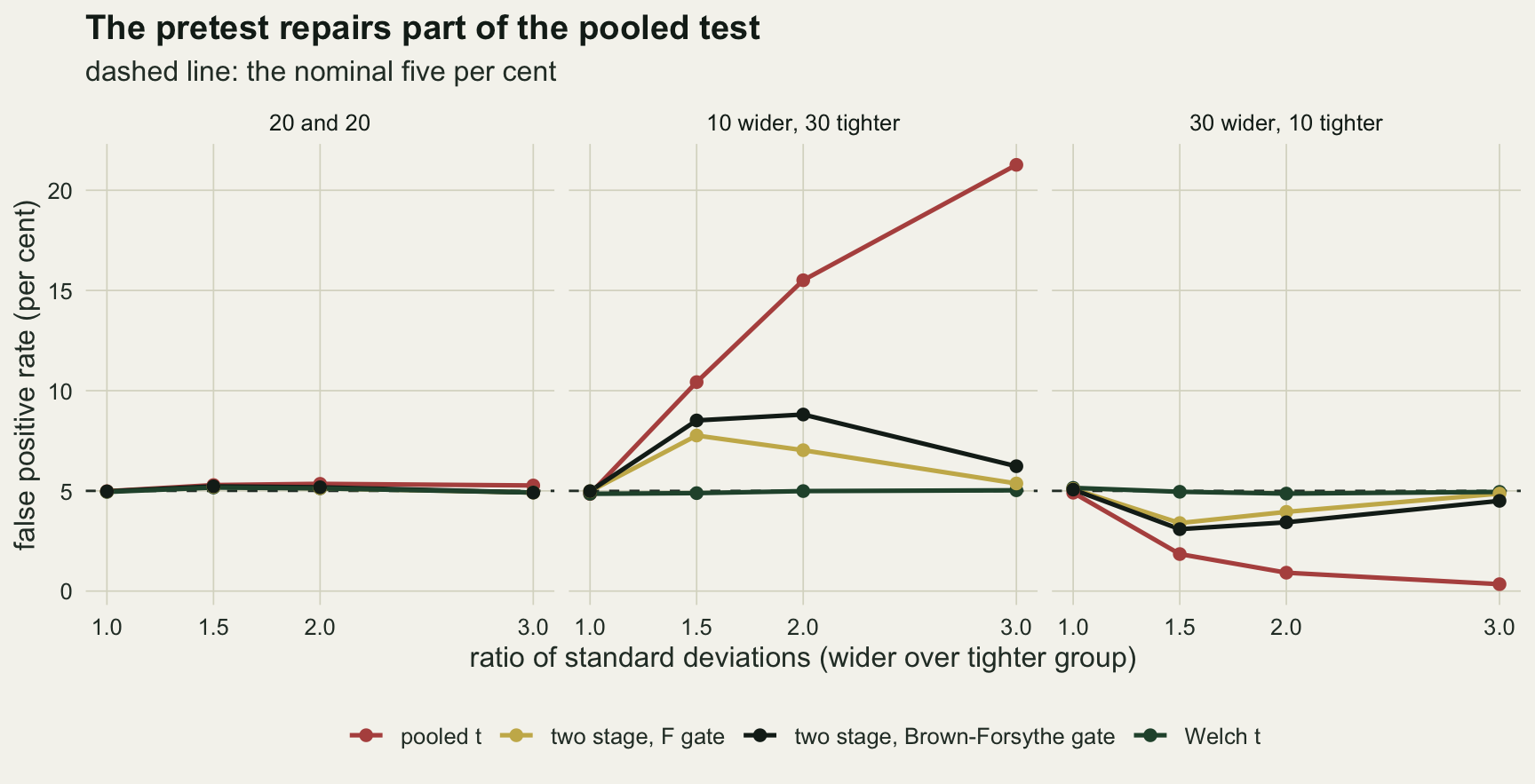
Passing the pretest makes the pooled test worse
The overall two stage rate mixes two kinds of dataset. In some, the pretest rejects and Welch runs; in the others, the pretest passes and the pooled test runs. A reader of a paper that says “variances did not differ (F test), so a pooled t test was used” is looking at a dataset of the second kind, and the relevant error rate for that paper is the pooled test’s rate among the datasets that passed. Its denominator is the number of datasets that passed, not the number simulated.
set.seed(6607)
focus <- sim_cell(10, 30, 2, 1, n_rep = n_rep)
f_pass    <- focus$p_f >= 0.05
n_f_pass  <- sum(f_pass)
share_f   <- 100 * n_f_pass / n_rep
rate_unc  <- 100 * mean(focus$p_pool < 0.05)
rate_cond <- 100 * mean(focus$p_pool[f_pass] < 0.05)
se_cond   <- sqrt(rate_cond * (100 - rate_cond) / n_f_pass)
rate_fail_pool  <- 100 * mean(focus$p_pool[!f_pass] < 0.05)
rate_fail_welch <- 100 * mean(focus$p_welch[!f_pass] < 0.05)
rate_two_focus  <- 100 * mean(ifelse(f_pass, focus$p_pool, focus$p_welch) < 0.05)
low_v1_pass <- 100 * mean(focus$v1_rel[f_pass] < 1)
low_v1_all  <- 100 * mean(focus$v1_rel < 1)
cond_mult <- rate_cond / 5

se_rel_pass <- median(focus$se_rel[f_pass])
se_rel_fail <- median(focus$se_rel[!f_pass])
se_rel_all  <- median(focus$se_rel)

cond_gap_sw <- grid_tab$cond_f[grid_tab$design == lab_sw] -
  grid_tab$pooled[grid_tab$design == lab_sw]
n_pass_sw3  <- pick(lab_sw, 3, "n_pass_f")
cond_sw3    <- pick(lab_sw, 3, "cond_f")
se_cond_sw3 <- sqrt(cond_sw3 * (100 - cond_sw3) / n_pass_sw3)
A fresh set of 40000 datasets for the pond design (ten wider, thirty tighter, ratio two) gives the pieces. The F test passed in 10159 of them, 25.4 per cent. Across all datasets the pooled test rejects in 15.5 per cent. Among the 10159 that passed the pretest, it rejects in 20.1 per cent, with a Monte Carlo standard error of 0.40 points: 4.0 times the nominal rate, and higher than the pooled test’s rate with no pretest at all. In the datasets that failed the pretest, Welch runs and rejects in 2.9 per cent. The two stage rate on this set of datasets, 7.2 per cent, is the average of those two branches weighted by how often each occurs: a high rate in a quarter of the datasets diluted by a low one in the rest.
The reason is in the standard error. Under normal data the difference in sample means is independent of the two sample variances, so the numerator of the t statistic knows nothing about the pretest. The denominator does. The datasets that pass are the ones whose sample variances happened to come out alike, and with a true ratio of two that almost always means the small, variable group produced a sample variance below its true value: that happened in 99.1 per cent of the passing datasets, against 56.3 per cent of all datasets. The pooled standard error is already too small in this design, and the selection makes it smaller. Expressed as a fraction of the true standard error of the difference, the median pooled standard error is 0.713 over all datasets, 0.644 in the datasets that passed, and 0.738 in the ones that failed.
The same ordering holds in every cell of the grid where the small group is the variable one and the variances differ, using the grid’s own datasets. The conditional rate minus the unconditional pooled rate is 0.8, 4.3 and 14.6 percentage points at ratios of 1.5, 2 and 3. The last of those rests on only 1085 passing datasets, so its standard error is 1.46 points, but a pretest that almost never passes at that ratio passes in exactly the wrong datasets when it does.
sw_tab <- grid_tab[grid_tab$design == lab_sw, ]
cond_long <- rbind(
  data.frame(sd_ratio = sw_tab$sd_ratio, rate = sw_tab$pooled,
             n_den = n_rep, what = "all datasets"),
  data.frame(sd_ratio = sw_tab$sd_ratio, rate = sw_tab$cond_f,
             n_den = sw_tab$n_pass_f, what = "passed F test"),
  data.frame(sd_ratio = sw_tab$sd_ratio, rate = sw_tab$cond_bf,
             n_den = sw_tab$n_pass_bf, what = "passed Brown-Forsythe"))
cond_long$se <- sqrt(cond_long$rate * (100 - cond_long$rate) / cond_long$n_den)
cond_long$what <- factor(cond_long$what,
                         levels = c("all datasets", "passed F test",
                                    "passed Brown-Forsythe"))

p_cond <- ggplot(cond_long, aes(sd_ratio, rate, colour = what)) +
  geom_hline(yintercept = 5, linetype = "dashed", colour = te_body,
             linewidth = 0.5) +
  geom_line(linewidth = 0.9) +
  geom_errorbar(aes(ymin = rate - 1.96 * se, ymax = rate + 1.96 * se),
                width = 0.06, linewidth = 0.5) +
  geom_point(size = 2) +
  scale_colour_manual(values = c(te_forest, te_rust, te_gold), name = NULL) +
  guides(colour = guide_legend(nrow = 2)) +
  scale_x_continuous(breaks = sd_grid) +
  labs(x = "ratio of standard deviations",
       y = "pooled t false positive rate (per cent)",
       title = "Conditioning on a pass") +
  theme_datasheet() +
  theme(legend.position = "bottom")

se_df <- data.frame(se_rel = focus$se_rel,
                    outcome = ifelse(f_pass, "F test passed", "F test rejected"))
p_se <- ggplot(se_df, aes(se_rel, fill = outcome)) +
  geom_density(alpha = 0.55, colour = NA) +
  geom_vline(xintercept = 1, linetype = "dashed", colour = te_ink,
             linewidth = 0.6) +
  scale_fill_manual(values = c(te_rust, te_forest), name = NULL) +
  guides(fill = guide_legend(nrow = 2)) +
  labs(x = "pooled SE / true SE of the difference", y = "density",
       title = "Why: the denominator") +
  theme_datasheet() +
  theme(legend.position = "bottom")

(p_cond | p_se) + plot_annotation(theme = theme_datasheet())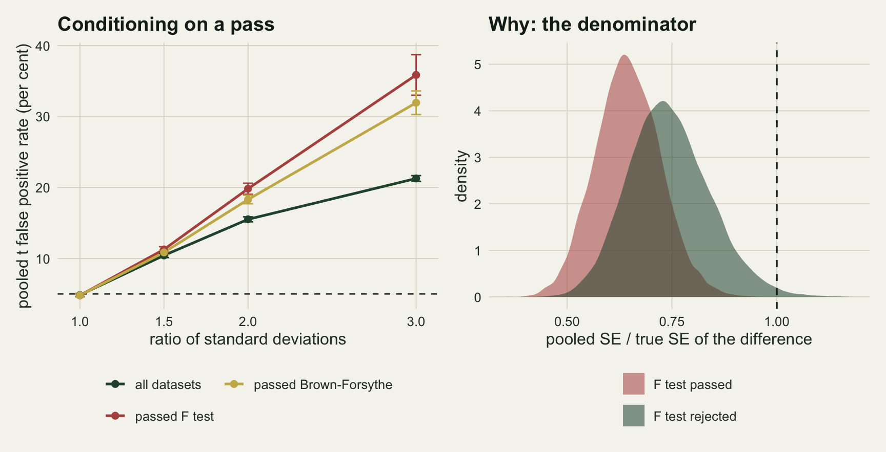
A pass is not evidence of equal variances
The share of datasets that pass is the pretest’s failure to detect a real difference. At a ratio of 1.5 with ten and thirty ponds, the F test passes in 63.9 per cent of datasets and the Brown-Forsythe test in 74.9 per cent. At a ratio of two the figures are 25.2 and 40.0 per cent. A standard deviation half as large again in one group is a big difference for a t test and a small one for a variance test on ten observations, and the rule treats the variance test’s silence as permission.
The Brown-Forsythe gate is the weaker detector of the two on normal data, which is the price of its insensitivity to skew, so it passes more often and lets more datasets through to the pooled test. Zimmerman (2004) ran the two stage procedure with Levene’s test as the gate over a range of unequal sample sizes and variances, found that it did not protect the significance level, and recommended the Welch test unconditionally whenever sample sizes are unequal, rather than only when the pretest rejects. This is the variance version of the argument in Testing for no effect: a non-significant pretest is compatible with equal variances and equally compatible with a pretest too small to see the difference.
What always-Welch costs when the variances are equal
The case for the two stage rule is power. If the variances really are equal, the pooled test has more degrees of freedom than Welch and should detect a real difference slightly more often, and the pretest is supposed to capture that gain when it is available. The cost of giving it up was measured directly: equal standard deviations, a true difference in means of 0.25, 0.5, 0.75 or 1 standard deviation, and the balanced and the ten and thirty allocations. With equal variances the thirty and ten allocation is the ten and thirty one with the groups relabelled, so it is not run twice. The pooled, Welch and two stage tests are applied to the same datasets, and the standard error of each difference in power is computed from the paired indicators.
delta_grid <- c(0.25, 0.5, 0.75, 1)
set.seed(8830)
pow_rows <- list()
for (j in 1:2) {
  for (d_shift in delta_grid) {
    res  <- sim_cell(design_df$n1[j], design_df$n2[j], 1, 1, delta = d_shift,
                     n_rep = n_rep)
    rej_pool  <- res$p_pool < 0.05
    rej_welch <- res$p_welch < 0.05
    rej_two   <- ifelse(res$p_f >= 0.05, res$p_pool, res$p_welch) < 0.05
    pow_rows[[length(pow_rows) + 1]] <- data.frame(
      design = design_df$label[j], delta = d_shift,
      pooled = 100 * mean(rej_pool), welch = 100 * mean(rej_welch),
      two_f  = 100 * mean(rej_two),
      loss_welch = 100 * mean(rej_pool - rej_welch),
      se_welch   = 100 * sd(rej_pool - rej_welch) / sqrt(n_rep),
      loss_two   = 100 * mean(rej_pool - rej_two),
      se_two     = 100 * sd(rej_pool - rej_two) / sqrt(n_rep),
      dfw_med    = median(res$df_w),
      dfw_big    = median(res$df_w[res$v1_big]),
      dfw_small  = median(res$df_w[!res$v1_big]))
  }
}
pow_tab <- do.call(rbind, pow_rows)

pw_pick <- function(des, d_shift, col) {
  pow_tab[pow_tab$design == des & pow_tab$delta == d_shift, col]
}
bal_loss_max <- max(pow_tab$loss_welch[pow_tab$design == lab_bal])
bal_se_max   <- max(pow_tab$se_welch[pow_tab$design == lab_bal])
sw_loss_max  <- max(pow_tab$loss_welch[pow_tab$design == lab_sw])
sw_loss_at   <- pow_tab$delta[pow_tab$design == lab_sw][
  which.max(pow_tab$loss_welch[pow_tab$design == lab_sw])]
sw_se_at     <- pow_tab$se_welch[pow_tab$design == lab_sw][
  which.max(pow_tab$loss_welch[pow_tab$design == lab_sw])]
sw_two_at    <- pow_tab$loss_two[pow_tab$design == lab_sw][
  which.max(pow_tab$loss_welch[pow_tab$design == lab_sw])]
sw_pool_at   <- pw_pick(lab_sw, sw_loss_at, "pooled")
sw_welch_at  <- pw_pick(lab_sw, sw_loss_at, "welch")
two_loss_max <- max(abs(pow_tab$loss_two))
lvl_welch_sw <- pick(lab_sw, 1, "welch")
lvl_pool_sw  <- pick(lab_sw, 1, "pooled")
lvl_two_sw   <- pick(lab_sw, 1, "two_f")
df_pool_sw   <- design_df$n1[2] + design_df$n2[2] - 2
dfw_med_at   <- pw_pick(lab_sw, sw_loss_at, "dfw_med")
dfw_big_at   <- pw_pick(lab_sw, sw_loss_at, "dfw_big")
dfw_small_at <- pw_pick(lab_sw, sw_loss_at, "dfw_small")
two_loss_lo  <- pw_pick(lab_sw, min(delta_grid), "loss_two")
two_se_lo    <- pw_pick(lab_sw, min(delta_grid), "se_two")
With twenty ponds in each group, always using Welch costs at most 0.14 percentage points of power across the four differences, against a paired Monte Carlo standard error no larger than 0.02. For practical purposes that is nothing, because with equal group sizes the Welch degrees of freedom stay near their maximum whenever the sample variances are similar.
With ten and thirty ponds the cost is not nothing. Of the four differences it is largest at 1.00 standard deviations, where the pooled test detects the difference in 76.0 per cent of datasets and Welch in 72.7 per cent: a loss of 3.34 points with a standard error of 0.14. The two stage rule recovers nearly all of it, losing only 0.42 points against the pooled test at the same difference. None of the Welch loss comes from a lower level: under the null with equal variances and this allocation, the grid above gave Welch 4.86 per cent and the pooled test 4.85 per cent. It is a loss of sensitivity, from the Welch degrees of freedom falling well below the pooled 38: at that difference their median was 15.8, and 13.5 in the datasets where the ten observation group had the larger sample variance against 18.7 in the rest. Part of the two stage rule’s recovery is level rather than sensitivity. On the same null datasets its rate was 4.98 per cent against the pooled test’s 4.85, and at the smallest difference, 0.25 standard deviations, its loss against the pooled test is -0.21 points (standard error 0.04): it rejects slightly more often than the exact test.
So the familiar claim that always using Welch costs nothing is only half true here. In a balanced design the pretest buys no power worth having. In an unbalanced design with a small group of ten it buys a few percentage points when the variances are truly equal, and it pays for them with the inflated false positive rates of the previous two sections when they are not and the small group is the more variable one. Which of those is the better trade depends on how sure the analyst is, before seeing the data, that the variances are equal; and a pretest on ten observations cannot supply that certainty.
loss_long <- rbind(
  data.frame(design = pow_tab$design, delta = pow_tab$delta,
             loss = pow_tab$loss_welch, se = pow_tab$se_welch,
             rule = "always Welch"),
  data.frame(design = pow_tab$design, delta = pow_tab$delta,
             loss = pow_tab$loss_two, se = pow_tab$se_two,
             rule = "two stage, F gate"))
loss_long$design <- factor(ifelse(loss_long$design == lab_bal, "20 and 20",
                                  "10 and 30"),
                           levels = c("20 and 20", "10 and 30"))

ggplot(loss_long, aes(delta, loss, colour = rule)) +
  geom_hline(yintercept = 0, colour = te_body, linewidth = 0.5) +
  geom_line(linewidth = 0.9) +
  geom_errorbar(aes(ymin = loss - 1.96 * se, ymax = loss + 1.96 * se),
                width = 0.04, linewidth = 0.5) +
  geom_point(size = 2) +
  facet_wrap(~ design, nrow = 1) +
  scale_colour_manual(values = c(te_forest, te_gold), name = NULL) +
  labs(x = "true difference in means (standard deviations)",
       y = "power lost vs pooled t (percentage points)",
       title = "The price of always using Welch",
       subtitle = "equal variances, so the pooled test is exact here") +
  theme_datasheet() +
  theme(legend.position = "bottom")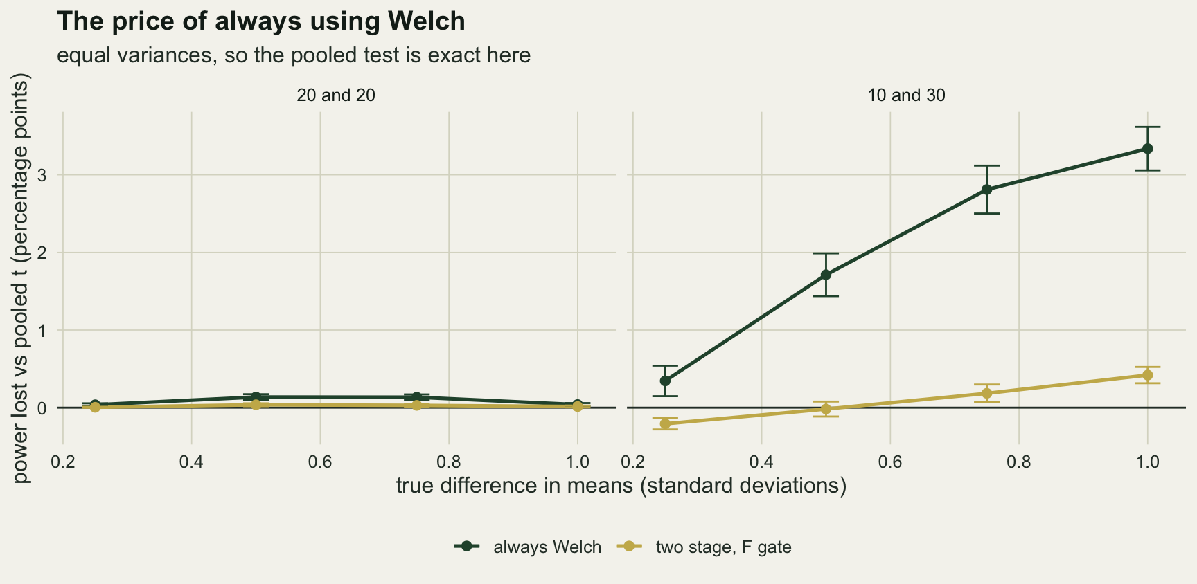
What to report
Use the Welch test without a pretest, and say so in the methods as a decision made before the data were seen: “means were compared with Welch’s t test, which does not assume equal variances”. That sentence carries its own justification and needs no preliminary test. It is what t.test does in R unless told otherwise, and Ruxton (2006) made the same recommendation to behavioural ecologists on the grounds that the unequal variance test loses little when variances are equal and is protected when they are not. The measurements above qualify the first half of that for small, unbalanced groups, where the loss was 3.3 points at its largest.
If a paper under review, or an old analysis of your own, used the two stage rule, the reported p value is from a procedure whose level is not the stated five per cent. In the pond design at a variance ratio of 1.5 the overall rate was 7.8 per cent, and the rate that applies to a dataset which passed the F test was 11.3 per cent. Rerunning the comparison with Welch on the same data is the cheap repair.
If the comparison is part of a larger linear model with several groups, where the equal variance assumption would otherwise come along silently, fit the unequal variance structure because the design says the groups differ (the varIdent model in modelling non-constant variance with nlme is one way to do that) and keep it whatever a test on the same data says, rather than letting a pretest decide. Rasch, Kubinger and Moder (2011) compared pretesting strategies for the two sample t test by simulation and reached the same recommendation: Welch, without a pretest.
When the group sizes are equal, the choice matters much less in both directions. The pooled test’s false positive rate stayed within 0.35 points of five at every variance ratio in the grid, and Welch’s power loss was negligible. Balanced allocation, where the field design allows it, removes most of the problem before any test is chosen.
Honest limits
Everything here is normal data. Under normality the sample mean and the sample variance are independent, which is what makes the mechanism so clean: the pretest selects on the denominator only. With skewed data the two are correlated, the F test loses its own level, and the Brown-Forsythe gate behaves differently from how it did here. The normality pretest version of the rule (Shapiro-Wilk, then t or Wilcoxon) was not simulated at all. Its logic is the same, a pretest chooses the test and the chosen test is then read as if no choice had been made, but its rates are not the ones measured above and the post makes no claim about them.
The grid has four variance ratios and three allocations of forty observations. The two stage rate peaked inside the grid, at a ratio of 1.5 with the F gate and between 1.5 and 2 with the Brown-Forsythe gate, and with no finer steps either peak could sit a little either side of where it was found, at a slightly higher rate. Smaller groups, which are common in field studies, give the pretest less power and would push the pass rates and the conditional rates higher; that direction is expected from the mechanism but was not measured.
Both the pretest and the main test use five per cent. Some texts recommend a more lenient pretest level, such as ten or twenty per cent, to catch more real differences. That shifts datasets from the pooled branch to the Welch branch and lowers the overall two stage rate, and the mechanism suggests the conditional problem remains, since whatever datasets still pass are still selected for similar sample variances; neither consequence was measured here.
The power comparison was run only with truly equal variances, because that is the only case in which the pooled test has its nominal level and a power comparison is fair. With unequal variances and a small variable group, the pooled test’s higher rejection rate under the alternative is partly the same inflation seen under the null and should not be read as power.
The Welch test itself is an approximation. Its level stayed within 0.17 points of five across this grid, but with very small groups, strong skew or ratios of standard deviations well beyond three it drifts, and Welch (1947) presented the degrees of freedom formula as an approximation, not an exact result.
References
Welch BL 1947 Biometrika 34(1-2):28-35 (10.1093/biomet/34.1-2.28)
Brown MB, Forsythe AB 1974 Journal of the American Statistical Association 69(346):364-367 (10.1080/01621459.1974.10482955)
Zimmerman DW 2004 British Journal of Mathematical and Statistical Psychology 57(1):173-181 (10.1348/000711004849222)
Ruxton GD 2006 Behavioral Ecology 17(4):688-690 (10.1093/beheco/ark016)
Rasch D, Kubinger KD, Moder K 2011 Statistical Papers 52(1):219-231 (10.1007/s00362-009-0224-x)