library(ggplot2)
library(patchwork)

te_paper  <- "#f5f4ee"
te_ink    <- "#16241d"
te_body   <- "#2c3a31"
te_forest <- "#275139"
te_rust   <- "#b5534e"
te_gold   <- "#c9b458"
te_line   <- "#dad9ca"

theme_datasheet <- function() {
  theme_minimal(base_size = 12) +
    theme(plot.background  = element_rect(fill = te_paper, colour = NA),
          panel.background = element_rect(fill = te_paper, colour = NA),
          panel.grid.major = element_line(colour = te_line, linewidth = 0.3),
          panel.grid.minor = element_blank(),
          text             = element_text(colour = te_body),
          plot.title       = element_text(colour = te_ink, face = "bold"),
          plot.subtitle    = element_text(colour = te_body),
          axis.text        = element_text(colour = te_body),
          strip.text       = element_text(colour = te_ink))
}Fitting an ODE: trajectory versus gradient matching
R
population dynamics
differential equations
model fitting
simulation
ecology tutorial
Fitting Lotka-Volterra ODEs to noisy counts in R: random starts miss the best fit half the time, and gradient matching gives a start that fails as samples thin.
Thirty years of a snowshoe hare index and a lynx index from the same valley, counted every spring. Both series cycle, the lynx peak trails the hare peak by a couple of years, and the obvious model is the one in every textbook: prey grow and are eaten, predators grow by eating and otherwise die. Written as two ordinary differential equations, Lotka and Volterra’s model has four rates, and fitting it to the counts is the natural first step before anything more realistic is tried. There is no closed-form solution to fit, so the rates have to come out of some combination of a numerical integrator and an optimiser, and the choice of combination matters more than it looks.
There are two standard ways to do it. Trajectory matching integrates the equations forward from a guessed starting state with guessed rates, compares the path with the data, and lets an optimiser move the rates and the starting state until the sum of squared differences is as small as it will go. Gradient matching never integrates anything. It smooths each series, differentiates the smooth, and regresses the estimated rate of change on the smoothed states; for the Lotka-Volterra model that regression is linear in all four rates. Varah proposed the spline version in 1982, Ellner, Seifu and Smith applied gradient matching to population time series in 2002, and Ramsay, Hooker, Campbell and Cao discuss in 2007 why the trajectory-matching sum of squares is so hard to minimise for oscillating systems. None of what follows is new. It is a measurement of those points on simulated data whose true rates are known, so that the chance of a failed fit and the bias of the shortcut can be put next to the sampling interval, the noise and the size of the cycle.
The site already fits one differential equation by integrating it. Stream metabolism from one oxygen logger integrates an oxygen budget forward from the first observation and minimises the squared difference, and its limits section reports that forty random starts converge to a single solution every time; a diel oxygen curve does not oscillate on its own, so that post never meets the problem here. The paradox of enrichment in R builds and checks a fixed-step Runge-Kutta integrator in logarithms for a predator-prey model but never confronts it with data. The theta-logistic model in R fits the one-step change in log abundance as a function of density, which is the discrete-time relative of gradient matching, and derivatives of a GAM trend differentiates a fitted smooth without any mechanistic model behind it. This post puts the two estimators side by side on a cycling model: how often trajectory matching finds its own best fit, why it fails when it fails, what gradient matching loses as the samples thin, and whether the shortcut is good enough to be the starting value for the real fit.
Lotka-Volterra in logarithms, with the step checked
p_true    <- c(a = 1, b = 0.1, c = 0.05, d = 0.6)
start_amp <- c(moderate = 20, large = 60, extreme = 150)
pred0     <- 5
t_end     <- 30
h_mod     <- 0.25
h_large   <- 0.1
h_fine    <- 0.002
dt_grid   <- c(0.25, 0.5, 1, 2)
sd_grid   <- c(0.05, 0.25)
eq_prey   <- p_true[["d"]] / p_true[["c"]]
eq_pred   <- p_true[["a"]] / p_true[["b"]]
small_per <- 2 * pi / sqrt(p_true[["a"]] * p_true[["d"]])
The model is written for the logarithms of prey density N and predator density P, because counts are compared on the log scale and because a log state cannot go negative in a trough. The prey log density changes at a minus b times P, and the predator log density at c times N minus d. The true rates are fixed at a = 1, b = 0.1, c = 0.05 and d = 0.6 per year, so the equilibrium is 12 prey and 10 predators, and small oscillations around it have a period of 8.11 years. The predator starts at 5 in every run. The prey starts at 20, 60 or 150, and nothing else changes: in this model the starting point alone decides how large the cycle is, and larger cycles also last longer. These constants, the thirty-year series, the sampling intervals of a quarter, a half, one and two years, and the two noise levels (a standard deviation of 0.05 or 0.25 on the log scale, independent for each count) were fixed before any fit was run.
The integrator is the classical fourth-order Runge-Kutta scheme with a fixed step, written once for a single path and once vectorised over the columns of a parameter matrix, so that one pass through the loop evaluates the sum of squares for many parameter sets at once. The vectorised version is what makes the optimisation affordable: the gradient for the optimiser is a forward difference, and all seven evaluations it needs go through the loop together. A trajectory that leaves the log range of plus or minus 30 is marked as a failure and given a sum of squares of a million. Gradient matching uses smooth.spline with all knots and its default generalised cross-validation, and reads the derivative at the sampling times from the same fit. The period of a series is estimated by counting upward crossings of the mean of its smooth.
lv_step <- function(u, v, a_r, b_r, c_r, d_r, hh) {
  a1 <- a_r - b_r * exp(v);              b1 <- c_r * exp(u) - d_r
  a2 <- a_r - b_r * exp(v + hh / 2 * b1); b2 <- c_r * exp(u + hh / 2 * a1) - d_r
  a3 <- a_r - b_r * exp(v + hh / 2 * b2); b3 <- c_r * exp(u + hh / 2 * a2) - d_r
  a4 <- a_r - b_r * exp(v + hh * b3);     b4 <- c_r * exp(u + hh * a3) - d_r
  list(u = u + hh / 6 * (a1 + 2 * a2 + 2 * a3 + a4),
       v = v + hh / 6 * (b1 + 2 * b2 + 2 * b3 + b4))
}
lv_path <- function(par, s_log, dt, n_obs, h) {
  k_sub <- max(1, round(dt / h)); hh <- dt / k_sub
  out <- matrix(NA_real_, n_obs, 2); out[1, ] <- s_log
  st <- list(u = s_log[1], v = s_log[2])
  for (i in 2:n_obs) {
    for (j in seq_len(k_sub)) st <- lv_step(st$u, st$v, par[1], par[2], par[3], par[4], hh)
    out[i, ] <- c(st$u, st$v)
  }
  out
}
lv_sse <- function(theta, y_obs, dt, h) {
  k_sub <- max(1, round(dt / h)); hh <- dt / k_sub
  a_r <- exp(theta[1, ]); b_r <- exp(theta[2, ]); c_r <- exp(theta[3, ]); d_r <- exp(theta[4, ])
  st <- list(u = theta[5, ], v = theta[6, ])
  sse <- (st$u - y_obs[1, 1])^2 + (st$v - y_obs[1, 2])^2
  dead <- rep(FALSE, ncol(theta))
  for (i in 2:nrow(y_obs)) {
    for (j in seq_len(k_sub)) {
      u <- st$u; v <- st$v
      a1 <- a_r - b_r * exp(v);              b1 <- c_r * exp(u) - d_r
      a2 <- a_r - b_r * exp(v + hh / 2 * b1); b2 <- c_r * exp(u + hh / 2 * a1) - d_r
      a3 <- a_r - b_r * exp(v + hh / 2 * b2); b3 <- c_r * exp(u + hh / 2 * a2) - d_r
      a4 <- a_r - b_r * exp(v + hh * b3);     b4 <- c_r * exp(u + hh * a3) - d_r
      st$u <- u + hh / 6 * (a1 + 2 * a2 + 2 * a3 + a4)
      st$v <- v + hh / 6 * (b1 + 2 * b2 + 2 * b3 + b4)
    }
    blown <- !is.finite(st$u) | !is.finite(st$v) | abs(st$u) > 30 | abs(st$v) > 30
    if (any(blown)) { dead <- dead | blown; st$u[blown] <- 0; st$v[blown] <- 0 }
    sse <- sse + (st$u - y_obs[i, 1])^2 + (st$v - y_obs[i, 2])^2
  }
  sse[dead] <- 1e6
  sse
}
fit_traj <- function(start_par, y_obs, dt, h) {
  fn <- function(th) lv_sse(matrix(th, 6), y_obs, dt, h)
  gr <- function(th) {
    s_vec <- lv_sse(cbind(th, th + diag(6) * 1e-6), y_obs, dt, h)
    (s_vec[-1] - s_vec[1]) / 1e-6
  }
  optim(start_par, fn, gr, method = "BFGS", control = list(maxit = 500, reltol = 1e-12))
}
gm_fit <- function(times, y_obs, spar = NULL) {
  s1 <- smooth.spline(times, y_obs[, 1], spar = spar, all.knots = TRUE)
  s2 <- smooth.spline(times, y_obs[, 2], spar = spar, all.knots = TRUE)
  u <- predict(s1, times)$y; v <- predict(s2, times)$y
  du <- predict(s1, times, deriv = 1)$y; dv <- predict(s2, times, deriv = 1)$y
  c1 <- coef(lm(du ~ exp(v))); c2 <- coef(lm(dv ~ exp(u)))
  list(p = unname(c(c1[1], -c1[2], c2[2], -c2[1])), s = c(u[1], v[1]))
}
period_guess <- function(times, series) {
  sp <- smooth.spline(times, series, all.knots = TRUE)
  fine_t <- seq(0, t_end, by = 0.05)
  cen <- predict(sp, fine_t)$y; cen <- cen - mean(cen)
  n_f <- length(cen)
  up <- fine_t[which(cen[-1] > 0 & cen[-n_f] <= 0)]
  if (length(up) >= 2) mean(diff(up)) else t_end
}
n_chk <- t_end / 0.5 + 1
step_err <- sapply(names(start_amp), function(amp) {
s_log <- log(c(start_amp[[amp]], pred0))
ref <- lv_path(p_true, s_log, 0.5, n_chk, h_fine)
c(h25 = max(abs(lv_path(p_true, s_log, 0.5, n_chk, 0.25) - ref)),
h10 = max(abs(lv_path(p_true, s_log, 0.5, n_chk, 0.1) - ref)),
h05 = max(abs(lv_path(p_true, s_log, 0.5, n_chk, 0.05) - ref)))
})
s_mod_log <- log(c(start_amp[[1]], pred0))
off_err <- sapply(c(2, 3), function(f_rate) {
max(abs(lv_path(p_true * f_rate, s_mod_log, 0.5, n_chk, h_mod) -
lv_path(p_true * f_rate, s_mod_log, 0.5, n_chk, h_fine)))
})
paths <- lapply(start_amp, function(n0) {
pl <- lapply(dt_grid, function(dt) lv_path(p_true, log(c(n0, pred0)), dt, t_end / dt + 1, h_fine))
names(pl) <- dt_grid
pl
})
t_quarter <- seq(0, t_end, by = 0.25)
amp_tab <- data.frame(
amp = names(start_amp),
prey_fold = sapply(paths, function(pl) exp(diff(range(pl[["0.25"]][, 1])))),
prey_min = sapply(paths, function(pl) exp(min(pl[["0.25"]][, 1]))),
period = sapply(paths, function(pl) period_guess(t_quarter, pl[["0.25"]][, 1])))Each step was checked against a step of 0.002 years over the whole thirty-year run, at the true rates and at half-year checkpoints, so that every step tried fits a whole number of times between them. For the moderate cycle a step of a quarter year keeps the largest error in any log density at 0.00043, so that is the step used to fit it. The large cycle needs a step of a tenth (largest error 0.000076, against 0.012 with a quarter), and the extreme cycle a twentieth (0.00014); the extreme cycle is only used for gradient matching, which never integrates. The simulated data themselves come from the fine step.
On the true paths the prey density varies 7.4-fold over a moderate cycle, 215-fold over a large one and 369787-fold over an extreme one, and the counted periods are 8.65, 11.25 and 19.00 years. A moderate cycle is sampled 4.3 times per cycle at the two-year interval, and a large cycle 5.6 times. The extreme cycle is included as a limiting case for the bias of the shortcut; a prey trough of 0.00041 per unit area is not something a count index would record.
series_df <- do.call(rbind, lapply(c("moderate", "large"), function(amp) {
  pl <- paths[[amp]][["0.25"]]
  rbind(data.frame(amp = amp, time = t_quarter, logn = pl[, 1], species = "prey"),
        data.frame(amp = amp, time = t_quarter, logn = pl[, 2], species = "predator"))
}))
set.seed(301)
obs_df <- do.call(rbind, lapply(c("moderate", "large"), function(amp) {
  pl <- paths[[amp]][["2"]]
  t_two <- seq(0, t_end, by = 2)
  rbind(data.frame(amp = amp, time = t_two, logn = pl[, 1] + rnorm(nrow(pl), 0, 0.05), species = "prey"),
        data.frame(amp = amp, time = t_two, logn = pl[, 2] + rnorm(nrow(pl), 0, 0.05), species = "predator"))
}))
amp_lab <- c(moderate = "moderate cycle: prey starts at 20", large = "large cycle: prey starts at 60")
series_df$amp <- factor(amp_lab[series_df$amp], levels = amp_lab)
obs_df$amp <- factor(amp_lab[obs_df$amp], levels = amp_lab)
ggplot(series_df, aes(time, logn, colour = species)) +
  geom_line(linewidth = 0.8) +
  geom_point(data = obs_df, size = 1.9) +
  facet_wrap(~ amp, ncol = 1) +
  scale_colour_manual(values = c(prey = te_forest, predator = te_rust), name = NULL) +
  labs(x = "time (years)", y = "log density",
       title = "Two orbits of the same predator-prey model",
       subtitle = "lines: the true path; points: one sample every 2 years, log-scale noise sd 0.05") +
  theme_datasheet() +
  theme(legend.position = "bottom")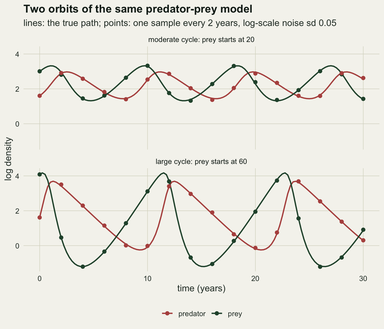
The sum of squares has a basin for every cycle count
Multiplying all four rates by the same factor leaves the shape of the orbit untouched and speeds the whole clock up by that factor. That gives a one-line slice through the six-dimensional surface which trajectory matching has to search: hold the starting state at its true value, multiply the rates by factors from a third to three, and compute the sum of squares for one dataset of the moderate cycle sampled every half year with noise sd 0.05.
set.seed(1812)
dt_slice <- 0.5
times_slice <- seq(0, t_end, by = dt_slice)
y_slice <- paths$moderate[["0.5"]] + matrix(rnorm(2 * length(times_slice), 0, 0.05), ncol = 2)
f_grid <- exp(seq(log(1 / 3), log(3), length.out = 500))
theta_slice <- rbind(matrix(log(p_true), 4, length(f_grid)) +
                       matrix(log(f_grid), 4, length(f_grid), byrow = TRUE),
                     log(start_amp[["moderate"]]), log(pred0))
sse_slice <- lv_sse(theta_slice, y_slice, dt_slice, 0.05)
n_f <- length(f_grid)
loc_min <- which(diff(sign(diff(sse_slice))) > 0) + 1
loc_max <- which(diff(sign(diff(sse_slice))) < 0) + 1
i_best  <- which.min(sse_slice)
f_best  <- f_grid[i_best]
basin_lo <- f_grid[max(loc_max[loc_max < i_best])]
basin_hi <- f_grid[min(loc_max[loc_max > i_best])]
other_min <- loc_min[loc_min != i_best]
sse_ratio_min <- min(sse_slice[other_min]) / sse_slice[i_best]
slice_minima <- function(h) {
  s_h <- lv_sse(theta_slice, y_slice, dt_slice, h)
  f_grid[which(diff(sign(diff(s_h))) > 0) + 1]
}
min_h_mod  <- slice_minima(h_mod)
min_h_fine <- slice_minima(h_fine)
n_min_moved <- if (length(min_h_mod) == length(min_h_fine)) sum(min_h_mod != min_h_fine) else NA
shift_steps <- max(abs(match(min_h_mod, f_grid) - match(min_h_fine, f_grid)))
set.seed(77)
box_log <- log(3)
rate_draw <- exp((runif(1e5, -box_log, box_log) + runif(1e5, -box_log, box_log)) / 2)
p_in_basin <- mean(rate_draw > basin_lo & rate_draw < basin_hi)
The deepest point of the slice sits at a factor of 0.998. Around it the central basin runs from 0.790 to 1.206, and outside it the slice has 9 further local minima, at factors where the fitted path fits a different whole number of cycles, or a shifted phase, into the thirty years. The best of those false minima has a sum of squares 230 times the best point of the slice, so nothing about them is a near tie: they are plainly wrong fits that an optimiser has no local reason to leave.
That basin width can be set against a common way of choosing starting values: each rate drawn independently from a threefold box around its true value, uniform on the log scale. The quantity the slice measures, the square root of a times d, then falls inside the central basin with probability 0.348. That is a one-line calculation on a six-dimensional problem, since b, c and the starting state move too, and the next section measures the real rate.
slice_df <- data.frame(f = f_grid, sse = sse_slice)
ggplot(slice_df, aes(f, sse)) +
  geom_vline(xintercept = c(basin_lo, basin_hi), linetype = "dashed", colour = te_gold, linewidth = 0.6) +
  geom_line(colour = te_ink, linewidth = 0.8) +
  geom_point(data = slice_df[other_min, ], colour = te_rust, size = 2.4) +
  geom_point(data = slice_df[i_best, ], colour = te_forest, size = 3) +
  scale_x_log10(breaks = c(1 / 3, 0.5, 1, 2, 3), labels = c("1/3", "1/2", "1", "2", "3")) +
  scale_y_log10() +
  labs(x = "all four rates multiplied by (log scale)", y = "sum of squares (log scale)",
       title = "One basin per cycle count",
       subtitle = "green: the best point; red: local minima; dashed gold: edges of the central basin") +
  theme_datasheet()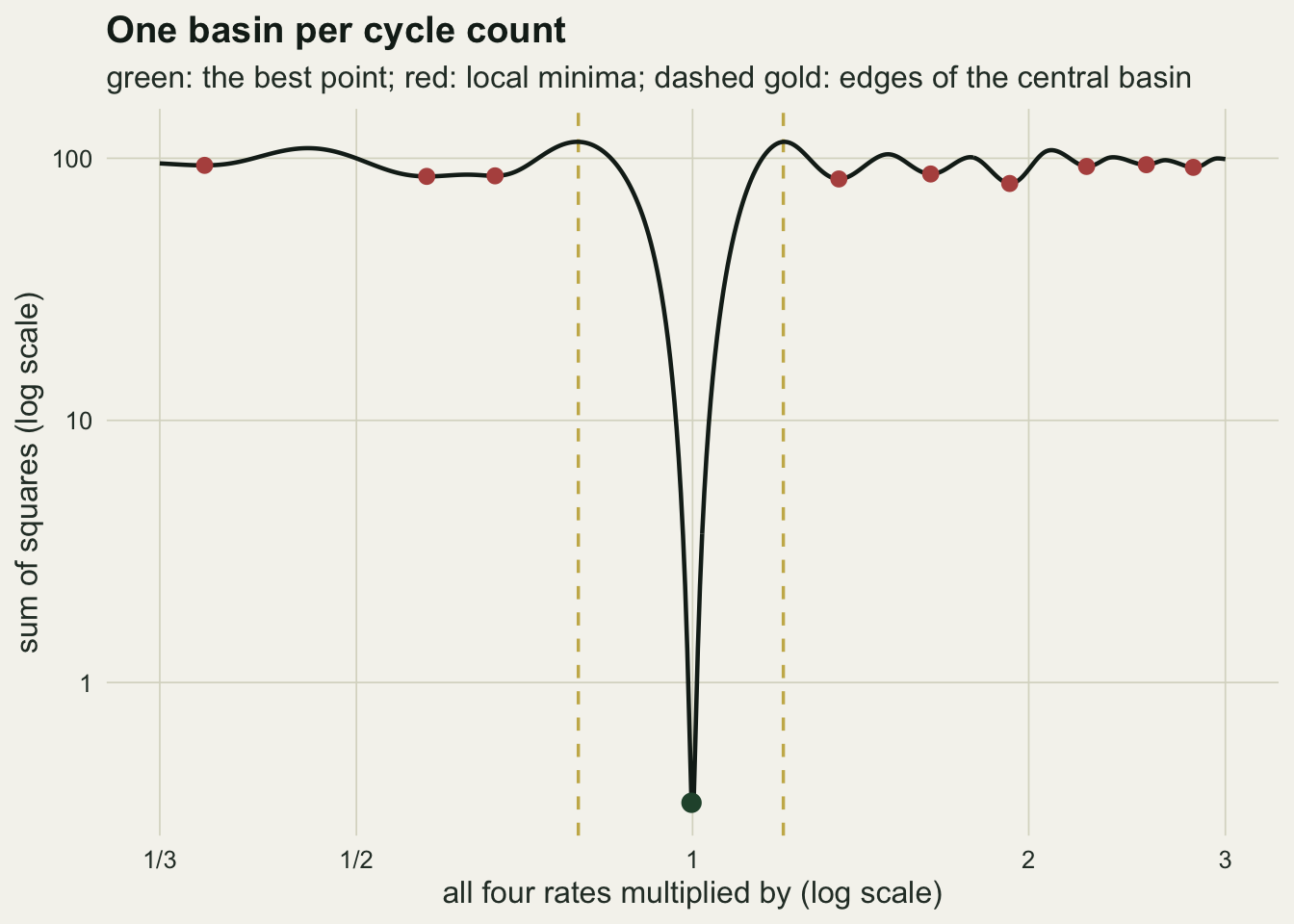
Random starts in a threefold box
n_data <- 8
n_rand <- 5
n_eq   <- 2
tol_rel <- 1e-3
rate_true <- sqrt(p_true[["a"]] * p_true[["d"]])
fit_dataset <- function(y_obs, times, dt, h, s_true, n_rand, n_eq, sd_obs) {
  gm <- gm_fit(times, y_obs)
  m_prey <- mean(exp(y_obs[, 1])); m_pred <- mean(exp(y_obs[, 2]))
  starts <- list(truth = c(log(p_true), s_true))
  for (i in seq_len(n_rand))
    starts[[paste0("random", i)]] <- c(log(p_true) + runif(4, -box_log, box_log), y_obs[1, ])
  for (i in seq_len(n_eq)) {
    r0 <- rate_true * exp(runif(1, -box_log, box_log))
    starts[[paste0("equilibrium", i)]] <- c(log(c(r0, r0 / m_pred, r0 / m_prey, r0)), y_obs[1, ])
  }
  r_per <- 2 * pi / period_guess(times, y_obs[, 1])
  starts$period <- c(log(c(r_per, r_per / m_pred, r_per / m_prey, r_per)), y_obs[1, ])
  starts$gradient <- c(log(pmax(gm$p, 1e-3)), gm$s)
  fits <- lapply(starts, fit_traj, y_obs = y_obs, dt = dt, h = h)
  sse <- vapply(fits, function(f) f$value, 0)
  best <- which.min(sse)
  sse_true <- lv_sse(matrix(c(log(p_true), s_true), 6), y_obs, dt, h)
  list(starts = data.frame(start = names(starts), type = sub("[0-9]+$", "", names(starts)),
                           sse = sse, rel = sse / sse[best], hit = sse <= sse[best] * (1 + tol_rel),
                           rate = vapply(fits, function(f) exp((f$par[1] + f$par[4]) / 2), 0) / rate_true,
                           conv = vapply(fits, function(f) f$convergence, 0)),
       est = data.frame(gm_a = gm$p[1] / p_true[["a"]], gm_d = gm$p[4] / p_true[["d"]],
                        tm_a = exp(fits[[best]]$par[1]) / p_true[["a"]],
                        tm_d = exp(fits[[best]]$par[4]) / p_true[["d"]],
                        gap_true = (sse_true - sse[best]) / sd_obs^2))
}
set.seed(2718)
start_list <- list(); est_list <- list()
for (dt in dt_grid) for (sd_obs in sd_grid) {
  times <- seq(0, t_end, by = dt)
  path <- paths$moderate[[as.character(dt)]]
  for (r in seq_len(n_data)) {
    y_obs <- path + matrix(rnorm(length(path), 0, sd_obs), ncol = 2)
    out <- fit_dataset(y_obs, times, dt, h_mod, path[1, ], n_rand, n_eq, sd_obs)
    start_list[[length(start_list) + 1]] <- cbind(amp = "moderate", dt = dt, sd_obs = sd_obs, dataset = r, out$starts)
    est_list[[length(est_list) + 1]] <- cbind(amp = "moderate", dt = dt, sd_obs = sd_obs, dataset = r, out$est)
  }
}
starts_mod <- do.call(rbind, start_list)
est_mod <- do.call(rbind, est_list)
For each sampling interval and noise level, 8 datasets were simulated from the moderate cycle. Every dataset was fitted from 5 random starts in the threefold box, with the starting state set to the first observation, and from five other starts that the next sections use: the true values, two starts that get the equilibrium ratios right from the series means but draw the overall rate at random from the same threefold box, one start that also counts the period, and the gradient-matching estimate. The optimiser is BFGS on the log rates with up to 500 iterations. A fit counts as reaching the best fit when its sum of squares is within one part in a thousand of the smallest found for that dataset by any of the starts, so success is relative to the best optimum found rather than to a certified global one.
ds_rate <- aggregate(hit ~ amp + dt + sd_obs + dataset + type, data = starts_mod, FUN = mean)
cell_rate <- aggregate(hit ~ amp + dt + sd_obs + type, data = ds_rate, FUN = mean)
cell_se <- aggregate(hit ~ amp + dt + sd_obs + type, data = ds_rate, FUN = function(x) sd(x) / sqrt(length(x)))
cell_rate$se <- cell_se$hit
pick_rate <- function(tab, type, dt, sd_obs, what = "hit") {
  tab[[what]][tab$type == type & tab$dt == dt & tab$sd_obs == sd_obs]
}
rand_all <- mean(starts_mod$hit[starts_mod$type == "random"])
rand_min <- min(cell_rate$hit[cell_rate$type == "random"])
rand_max <- max(cell_rate$hit[cell_rate$type == "random"])
eq_all   <- mean(starts_mod$hit[starts_mod$type == "equilibrium"])
truth_all <- mean(starts_mod$hit[starts_mod$type == "truth"])
n_blown  <- sum(starts_mod$sse >= 1e6)
n_nonconv <- sum(starts_mod$conv != 0)
n_fits_mod <- nrow(starts_mod)
miss <- starts_mod[!starts_mod$hit & starts_mod$sse < 1e6, ]
miss_in_basin <- sum(miss$rate > basin_lo & miss$rate < basin_hi)
miss_rel_lo <- tapply(miss$rel, miss$sd_obs, min)
miss_rel_hi <- tapply(miss$rel, miss$sd_obs, max)
Across the 640 fits, 3 stopped at the iteration limit and none ran off to infinity, so the failures below are not a budget artefact. The start at the true values reached the best fit in 100 per cent of datasets. Random starts in the threefold box reached it in 51.6 per cent of fits overall, and between 35.0 and 62.5 per cent in the individual cells, where a cell’s standard error across its datasets runs up to 0.096. At the two-year interval with little noise the rate was 35.0 per cent. The slice’s estimate of 0.348 was lower than what the full six-dimensional fit achieved, so the optimiser evidently reaches the central basin from some starts outside it by moving the other parameters as well.
Getting the equilibrium right does not help. The two starts with correct prey and predator means but a random overall rate reached the best fit in 36.7 per cent of fits, fewer than the fully random starts. The difficulty is along the clock, and the equilibrium says nothing about the clock.
The failures stop at other cycle counts, not near the truth. Of the 244 fits that missed, 0 had a fitted cycle rate inside the central basin of the slice. In the figure the missed fits sit in vertical bands, several of them close to the local minima of the slice, and in two horizontal bands that are only the noise level: with the noise sd at 0.05 a missed fit had a sum of squares between 115 and 241 times the best, and with the noise sd at 0.25, whose best fit is itself much worse, between 2.5 and 12.5 times.
miss_df <- starts_mod[starts_mod$type %in% c("random", "equilibrium") & starts_mod$sse < 1e6 &
                        starts_mod$rate > 0.1 & starts_mod$rate < 10, ]
n_miss_shown <- sum(!miss_df$hit)
miss_df$outcome <- ifelse(miss_df$hit, "reached the best fit", "stopped elsewhere")
ggplot(miss_df, aes(rate, rel, colour = outcome)) +
  geom_vline(xintercept = f_grid[other_min], linetype = "dotted", colour = te_body, linewidth = 0.5) +
  geom_jitter(width = 0.02, height = 0, size = 1.6, alpha = 0.7) +
  scale_x_log10(breaks = c(0.25, 0.5, 1, 2, 4), labels = c("1/4", "1/2", "1", "2", "4")) +
  scale_y_log10() +
  scale_colour_manual(values = c("reached the best fit" = te_forest, "stopped elsewhere" = te_rust), name = NULL) +
  labs(x = "fitted cycle rate, square root of a times d, over the true value (log scale)",
       y = "sum of squares over the best one (log scale)",
       title = "Failed fits stop at another cycle count",
       subtitle = "moderate cycle, all intervals and noise levels; dotted: minima of the slice") +
  theme_datasheet() +
  theme(legend.position = "bottom")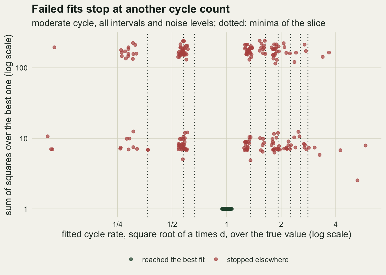
Gradient matching needs no start, and what it costs
n_gm <- 200
set.seed(4242)
gm_list <- list()
for (amp in names(start_amp)) for (dt in dt_grid) {
  times <- seq(0, t_end, by = dt)
  path <- paths[[amp]][[as.character(dt)]]
  exact <- gm_fit(times, path + matrix(rnorm(length(path), 0, 1e-5), ncol = 2), spar = 0.01)$p
  for (sd_obs in sd_grid) {
    est <- replicate(n_gm, gm_fit(times, path + matrix(rnorm(length(path), 0, sd_obs), ncol = 2))$p)
    gm_list[[length(gm_list) + 1]] <- data.frame(
      amp = amp, dt = dt, sd_obs = sd_obs,
      per_cycle = amp_tab$period[amp_tab$amp == amp] / dt,
      a_ratio = mean(est[1, ]) / p_true[["a"]], d_ratio = mean(est[4, ]) / p_true[["d"]],
      a_se = sd(est[1, ]) / sqrt(n_gm) / p_true[["a"]],
      a_exact = exact[1] / p_true[["a"]], d_exact = exact[4] / p_true[["d"]],
      n_neg = sum(est[1, ] <= 0 | est[4, ] <= 0))
  }
}
gm_tab <- do.call(rbind, gm_list)
gm_pick <- function(amp, dt, sd_obs, what) gm_tab[[what]][gm_tab$amp == amp & gm_tab$dt == dt & gm_tab$sd_obs == sd_obs]
a_se_max <- max(gm_tab$a_se)
Gradient matching replaces the search with two regressions. The smoothed prey log density has a derivative equal to a minus b times P, so regressing that derivative on the smoothed predator density gives a as the intercept and b as minus the slope; the predator equation gives c and d the same way. There is nothing to start and nothing to converge. The price is that the derivative of a smooth is not the derivative of the process, and every departure between the two goes straight into the rates. Each combination of cycle size, sampling interval and noise was simulated 200 times, and the discretisation part was isolated by fitting noise-free data with an almost interpolating spline.
On the moderate cycle with little noise gradient matching gets prey growth right while the samples are dense: the mean estimate is 0.991 of the true value at a half-year interval and 0.977 at one year. At two years, 4.3 samples per cycle, it falls to 0.810, and the noise-free interpolating spline gives 0.819, so almost all of that loss is discretisation: a spline cannot recover the slope of a cycle it sees four times per period. The largest Monte Carlo standard error of any mean ratio in the grid is 0.043.
set.seed(8080)
times_q <- seq(0, t_end, by = 0.25)
path_q <- paths$moderate[["0.25"]]
du_true <- p_true[["a"]] - p_true[["b"]] * exp(path_q[, 2])
split_est <- replicate(n_gm, {
  y_obs <- path_q + matrix(rnorm(length(path_q), 0, 0.25), ncol = 2)
  s_prey <- smooth.spline(times_q, y_obs[, 1], all.knots = TRUE)
  s_pred <- smooth.spline(times_q, y_obs[, 2], all.knots = TRUE)
  du_smooth <- predict(s_prey, times_q, deriv = 1)$y
  v_smooth <- predict(s_pred, times_q)$y
  c(both        = unname(coef(lm(du_smooth ~ exp(v_smooth)))[1]),
    deriv_only  = unname(coef(lm(du_smooth ~ exp(path_q[, 2])))[1]),
    state_only  = unname(coef(lm(du_true ~ exp(v_smooth)))[1]),
    deriv_slope = unname(coef(lm(du_smooth ~ du_true))[2]))
})
split_mean <- rowMeans(split_est) / c(p_true[["a"]], p_true[["a"]], p_true[["a"]], 1)
split_se <- apply(split_est, 1, sd) / sqrt(n_gm)
Noise adds a second bias that does not come from sparse sampling. With the noise sd at 0.25, prey growth comes out at 0.937 even at the quarter-year interval, where discretisation costs nothing, and at 0.855 at one year. The obvious suspect is the regressor, since the smoothed predator density carries error and a regressor measured with error pulls a slope towards zero. Splitting the regression at the quarter-year interval says otherwise. Regressing the true prey rate of change on the smoothed predator density gives 1.008 of the true prey growth, while regressing the spline’s derivative on the true predator density gives 0.939, against 0.954 when both come from the smooths as in the full method (all three on one fresh set of 200 datasets, standard errors up to 0.005). That last figure measures the same quantity as the 0.937 above on different simulated data, and the two differ by 2.6 combined standard errors, so the three numbers of the split are compared with each other and not with the grid. The loss is in the response. A spline fitted to noisy counts is smoother than the process, so its slopes are flatter than the true rates of change: regressed on the true rate of change, the spline’s derivative has a slope of 0.950, and a flattened response shrinks both the slope and the intercept of the gradient-matching regression.
spar_grid <- c(0.1, 0.3, 0.5, 0.7)
set.seed(5151)
spar_cells <- data.frame(dt = c(2, 1), sd_obs = c(0.05, 0.25))
spar_tab <- do.call(rbind, lapply(seq_len(nrow(spar_cells)), function(k) {
  dt <- spar_cells$dt[k]; sd_obs <- spar_cells$sd_obs[k]
  times <- seq(0, t_end, by = dt); path <- paths$moderate[[as.character(dt)]]
  ys <- replicate(100, path + matrix(rnorm(length(path), 0, sd_obs), ncol = 2), simplify = FALSE)
  data.frame(dt = dt, sd_obs = sd_obs, spar = spar_grid,
             a_ratio = sapply(spar_grid, function(sp) mean(sapply(ys, function(y) gm_fit(times, y, sp)$p[1]))))
}))
spar_best <- function(dt) max(spar_tab$a_ratio[spar_tab$dt == dt])
The choice of smoothing does not rescue either case. At the two-year interval with little noise, the best of four fixed smoothing parameters gave 0.812 of the true prey growth, against 0.810 from cross-validation, and heavier smoothing only made it worse (0.243 at a smoothing parameter of 0.5). At one year with the noise sd at 0.25 the best fixed value gave 0.824, below the 0.855 from cross-validation. The bias in these two cells is a property of the sampling and of the noise rather than of a badly chosen smoothing parameter.
The size of the cycle is the other axis, and it matters as much as the interval. At the one-year interval with little noise the mean prey growth estimate is 0.977 for the moderate cycle, 0.936 for the large one and 0.673 for the extreme one, even though the larger cycles are longer and so are sampled more often per cycle. A big cycle spends a short, steep stretch climbing out of each trough, and those stretches are the ones a spline through sparse points flattens. A single bias figure for gradient matching therefore describes one cycle shape, not the method.
gm_long <- rbind(
  data.frame(gm_tab[, c("amp", "dt", "sd_obs")], par = "prey growth a", ratio = gm_tab$a_ratio, exact = gm_tab$a_exact),
  data.frame(gm_tab[, c("amp", "dt", "sd_obs")], par = "predator death d", ratio = gm_tab$d_ratio, exact = gm_tab$d_exact))
gm_long$noise <- paste("noise sd", gm_long$sd_obs)
gm_long$amp <- factor(gm_long$amp, levels = names(start_amp))
gm_long$par <- factor(gm_long$par, levels = c("prey growth a", "predator death d"))
exact_long <- unique(gm_long[, c("amp", "dt", "par", "exact")])
ggplot(gm_long, aes(dt, ratio)) +
  geom_hline(yintercept = 1, colour = te_body, linewidth = 0.4) +
  geom_line(data = exact_long, aes(dt, exact), colour = te_ink, linetype = "dashed", linewidth = 0.6) +
  geom_line(aes(colour = noise), linewidth = 0.9) +
  geom_point(aes(colour = noise), size = 2) +
  facet_grid(par ~ amp) +
  scale_x_log10(breaks = dt_grid, labels = c("0.25", "0.5", "1", "2")) +
  scale_colour_manual(values = c(te_forest, te_rust), name = NULL) +
  labs(x = "sampling interval (years, log scale)", y = "mean estimate over true value",
       title = "Gradient matching loses the rate as samples thin",
       subtitle = "dashed: noise-free data through an interpolating spline, the discretisation part alone") +
  theme_datasheet() +
  theme(legend.position = "bottom")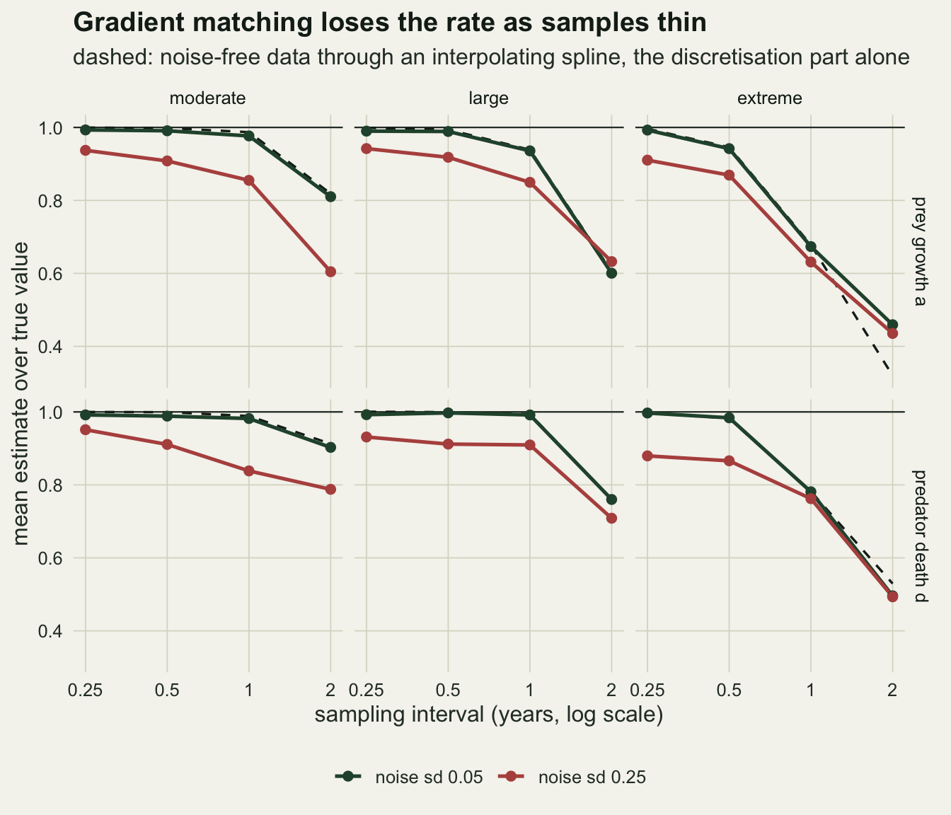
Gradient matching as the starting value
n_large <- 8
set.seed(6060)
start_list <- list(); est_list <- list()
for (dt in c(0.5, 2)) {
  times <- seq(0, t_end, by = dt)
  path <- paths$large[[as.character(dt)]]
  for (r in seq_len(n_large)) {
    y_obs <- path + matrix(rnorm(length(path), 0, 0.05), ncol = 2)
    out <- fit_dataset(y_obs, times, dt, h_large, path[1, ], n_rand, 0, 0.05)
    start_list[[length(start_list) + 1]] <- cbind(amp = "large", dt = dt, sd_obs = 0.05, dataset = r, out$starts)
    est_list[[length(est_list) + 1]] <- cbind(amp = "large", dt = dt, sd_obs = 0.05, dataset = r, out$est)
  }
}
starts_large <- do.call(rbind, start_list)
est_large <- do.call(rbind, est_list)
ds_large <- aggregate(hit ~ amp + dt + sd_obs + dataset + type, data = starts_large, FUN = mean)
rate_large <- aggregate(hit ~ amp + dt + sd_obs + type, data = ds_large, FUN = mean)
rate_large$se <- aggregate(hit ~ amp + dt + sd_obs + type, data = ds_large, FUN = function(x) sd(x) / sqrt(length(x)))$hit
tm_mod <- aggregate(cbind(gm_a, gm_d, tm_a, tm_d) ~ dt + sd_obs, data = est_mod, FUN = mean)
tm_large <- aggregate(cbind(gm_a, gm_d, tm_a, tm_d) ~ dt, data = est_large, FUN = mean)
gm_rate_mod  <- sqrt(tm_mod$gm_a * tm_mod$gm_d)
gm_rate_large <- sqrt(tm_large$gm_a * tm_large$gm_d)
per_rate <- small_per / amp_tab$period
names(per_rate) <- amp_tab$amp
tm_dev_max <- max(abs(c(tm_mod$tm_a, tm_mod$tm_d, tm_large$tm_a, tm_large$tm_d) - 1))
grad_all <- merge(rbind(starts_mod, starts_large)[rbind(starts_mod, starts_large)$type == "gradient", ],
                  rbind(est_mod, est_large))
grad_all$inside <- sqrt(grad_all$gm_a * grad_all$gm_d) > basin_lo & sqrt(grad_all$gm_a * grad_all$gm_d) < basin_hi
grad_in_hit  <- sum(grad_all$inside & grad_all$hit)
grad_in_n    <- sum(grad_all$inside)
grad_out_hit <- sum(!grad_all$inside & grad_all$hit)
grad_out_n   <- sum(!grad_all$inside)
truth_both <- mean(rbind(starts_mod, starts_large)$hit[rbind(starts_mod, starts_large)$type == "truth"])
n_data_both <- nrow(est_mod) + nrow(est_large)
gap_all <- c(est_mod$gap_true, est_large$gap_true)
gap_q99 <- qchisq(0.99, 6)
n_gap_over <- sum(gap_all > gap_q99)
tm_pick <- function(dt, sd_obs, what) tm_mod[[what]][tm_mod$dt == dt & tm_mod$sd_obs == sd_obs]
The practical recommendation that follows from the two sections above is to use the shortcut to find the basin and trajectory matching to finish the fit. The large cycle was fitted in the same way as the moderate one at the half-year and two-year intervals with the noise sd at 0.05, 8 datasets each, without the equilibrium-ratio starts.
Once trajectory matching reaches the best fit, its estimates are close to the truth: over all cells of both cycles the mean estimates of a and d differ from the true values by at most 0.045 as a proportion, including the two-year interval where gradient matching gave 0.626 for prey growth with the noise sd at 0.25.
On the moderate cycle the gradient-matching start reached the best fit in every dataset at intervals up to half a year at both noise levels, and at one year with little noise. It failed in 1 of 8 datasets at two years with little noise, and at two years with the noise sd at 0.25 it succeeded in only 25 per cent, below the random starts in the same cell (42.5 per cent). The reason is the slice. In that cell the mean gradient-matching estimates of a and d imply a cycle rate of 0.717 of the truth, outside the central basin that began at 0.790; at a half year with the same noise the implied rate is 0.941, inside it. The large cycle repeats the pattern: the gradient start succeeded in 100 per cent of datasets at a half year and 25 per cent at two years, where its implied rate was 0.671. Over both cycles, gradient starts whose implied rate fell inside the central basin reached the best fit in 61 of 62 datasets, and those outside it in 5 of 18. A biased shortcut works as a start while the cycle rate it implies stays inside the basin, with the basin edge a guide rather than a rule, since it was measured on one slice of one dataset.
Counting the period is a cheaper way to set the clock, and on the moderate cycle it reached the best fit in every one of the 64 datasets. It rests on the small-oscillation formula, which says the period is two pi over the square root of a times d, and that formula is exact only for small cycles. For the large cycle the counted period of 11.25 years implies a rate 0.721 of the truth, below the lower edge of the basin measured on the moderate slice, which need not be the basin of the large cycle, and the counted-period start reached the best fit in 50 per cent of datasets at a half year and 88 per cent at two years. Random starts on the large cycle reached it in 62.5 and 47.5 per cent of fits.
succ_df <- rbind(cell_rate, rate_large)
succ_df <- succ_df[succ_df$type != "truth", ]
succ_df$panel <- ifelse(succ_df$amp == "large", "large cycle, noise sd 0.05", paste("moderate cycle, noise sd", succ_df$sd_obs))
succ_df$panel <- factor(succ_df$panel, levels = c("moderate cycle, noise sd 0.05", "moderate cycle, noise sd 0.25", "large cycle, noise sd 0.05"))
start_lab <- c(random = "random, threefold box", equilibrium = "equilibrium ratios, random rate",
               period = "equilibrium ratios, counted period", gradient = "gradient matching")
succ_df$start <- factor(start_lab[succ_df$type], levels = start_lab)
ggplot(succ_df, aes(dt, hit, colour = start)) +
  geom_line(aes(linetype = start), linewidth = 0.8, position = position_dodge(width = 0.12)) +
  geom_errorbar(aes(ymin = pmax(0, hit - 2 * se), ymax = pmin(1, hit + 2 * se)), width = 0,
                linewidth = 0.5, position = position_dodge(width = 0.12)) +
  geom_point(aes(shape = start), size = 2.2, position = position_dodge(width = 0.12)) +
  facet_wrap(~ panel, ncol = 3) +
  scale_x_log10(breaks = dt_grid, labels = c("0.25", "0.5", "1", "2")) +
  scale_y_continuous(limits = c(0, 1)) +
  scale_colour_manual(values = c(te_rust, te_gold, te_ink, te_forest), name = NULL) +
  scale_linetype_manual(values = c("solid", "solid", "dashed", "solid"), name = NULL) +
  scale_shape_manual(values = c(16, 16, 17, 15), name = NULL) +
  guides(colour = guide_legend(nrow = 2), linetype = guide_legend(nrow = 2), shape = guide_legend(nrow = 2)) +
  labs(x = "sampling interval (years, log scale)", y = "share of fits reaching the best sum of squares",
       title = "Where each starting rule lands",
       subtitle = "8 datasets per point; bars: two standard errors across datasets") +
  theme_datasheet() +
  theme(legend.position = "bottom")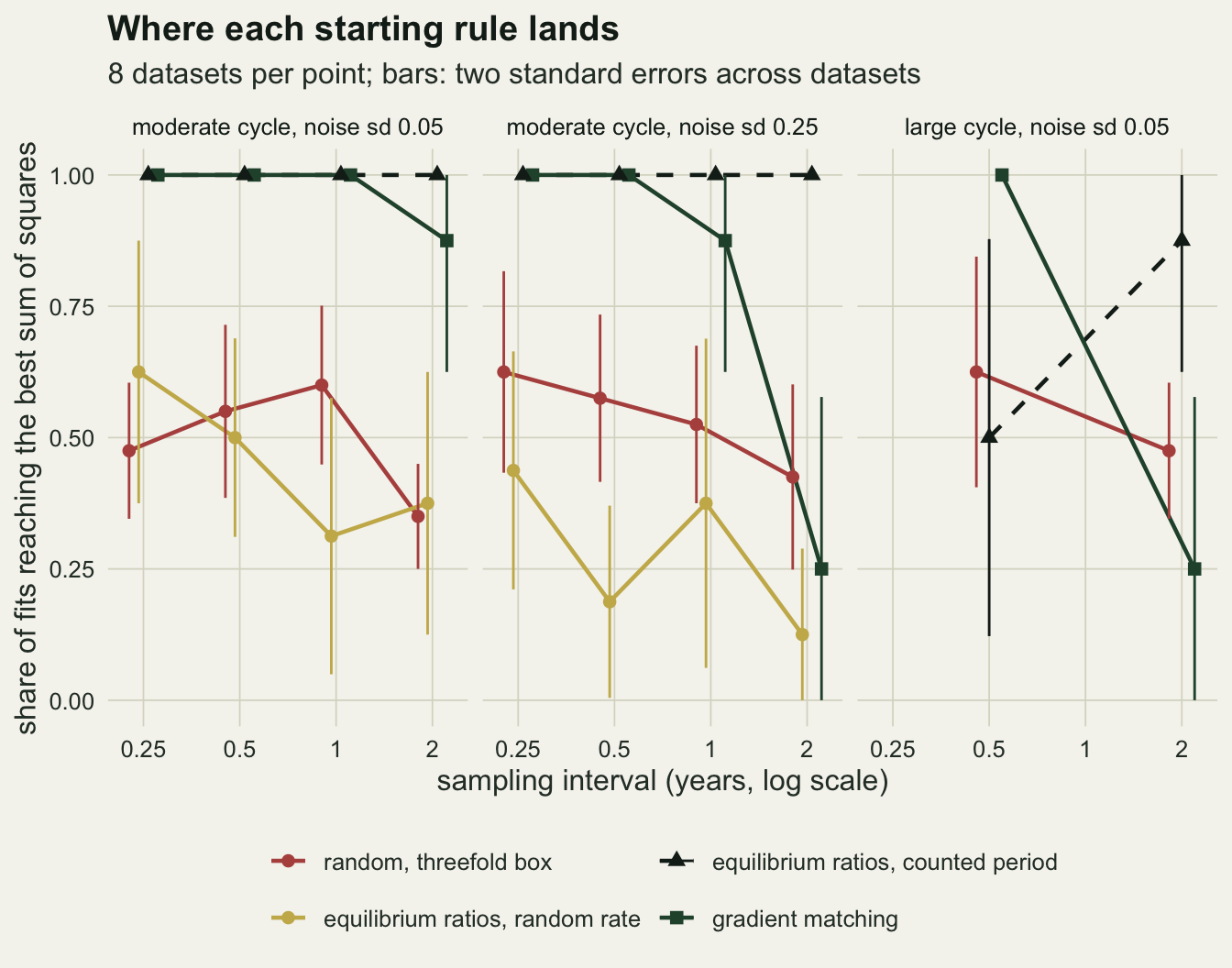
What to report
Report how the starting values were chosen and how many were tried, and report the sum of squares reached from each, not only the best parameter values. On a cycling model a fit from one start is a fit to whichever basin that start happened to be in, and in these simulations a random start in a threefold box landed in the right one about half the time. If several starts agree on the best sum of squares and the rest stop at clearly worse values, say so; that pattern is the signature of the problem here rather than a sign of a broken fit.
Do not report gradient-matching rates as the final estimates when the series is sparse or noisy. At four samples per cycle, or with a log-scale noise sd of 0.25, the prey growth rate from the shortcut was low by far more than its Monte Carlo error, and trajectory matching from a start in the right basin removed that bias. Use the shortcut as the start, then check whether the finished fit moved the implied cycle rate a long way; if it did, fit again from a start with the period counted and from a few random starts and keep the best.
State the sampling interval as samples per cycle and give the range of the counts over a cycle. Both the bias of gradient matching and the failure of the gradient start depend on those two quantities, and a reader cannot judge either from the number of observations alone.
Honest limits
The data come from the model that is fitted. The Lotka-Volterra model has no density dependence in the prey and no handling time in the predator, and real hare and lynx series follow it only loosely; with the wrong model the sum-of-squares surface changes and the basin measured here does not carry over. The noise is independent normal error on the log scale with no process noise, which is the case trajectory matching assumes. With process noise the integrated deterministic path drifts away from the data over thirty years while gradient matching only uses local slopes, so the comparison could shift in either direction; that was not simulated.
The basin was measured on one slice of one dataset, for the moderate cycle at the half-year interval. It is used as an explanation of which starts fail, not as a threshold. A longer series fits more cycles into the run and would be expected to narrow the basin, while the longer period of a large cycle would be expected to widen it; neither was measured.
Success is defined against the best sum of squares found by up to ten starts per dataset, one of them at the true values. That makes the definition generous to all starting rules: a dataset where every start missed a better optimum would count as a success for all of them. Two checks make that unlikely without proving it. The true-value start reached the best fit in 100 per cent of the 80 datasets of both cycles. And the sum of squares at the true values exceeded the best one found by between 0.83 and 16.6 times the noise variance, with a mean of 6.1. For a least-squares fit of six free quantities that difference behaves roughly like a chi-square variable with six degrees of freedom, whose mean is 6 and whose 99th percentile is 16.8, and 0 datasets went past that percentile. An optimum that every start missed would have to lie still further below the truth, a closer fit to the noise than noise alone tends to allow.
The integration step was checked at the true rates only. Away from them the quarter-year step used for the moderate cycle loses accuracy: at twice the true rates its largest error is 0.0116 in log density and at three times 0.257, so the sum of squares far out along the clock is only approximate. It does not move the landscape that matters here. Recomputed once at the quarter-year step and once at a step of 0.002, the slice has 10 and 10 local minima, the deepest included. The only one at a different factor is the deepest, and it moves by 1 point of the 500-point grid (1 minimum moved in all).
With 8 datasets per cell the success rates of single starting rules move in steps of one eighth, and the difference between the gradient start and the random starts in the worst cell rests on a small number of datasets. The cells were not enlarged because each fit is an optimisation over a numerical integral and the post has to knit in a few minutes.
Generalised profiling, the method Ramsay and colleagues proposed, is the obvious third estimator: it fits a smooth that is penalised for departing from the differential equation and so sits between the two methods here. It was not implemented. Neither were multiple shooting, which restarts the integration at several points in the series and flattens the false basins, nor Bayesian fits, which face the same multimodality in the posterior.
References
Varah JM 1982 SIAM Journal on Scientific and Statistical Computing 3(1):28-46 (10.1137/0903003)
Ellner SP, Seifu Y, Smith RH 2002 Ecology 83(8):2256-2270 (10.1890/0012-9658(2002)083[2256:FPDMTT]2.0.CO;2)
Ramsay JO, Hooker G, Campbell D, Cao J 2007 Journal of the Royal Statistical Society Series B 69(5):741-796 (10.1111/j.1467-9868.2007.00610.x)