library(ggplot2)
library(patchwork)

te_paper  <- "#f5f4ee"
te_ink    <- "#16241d"
te_body   <- "#2c3a31"
te_forest <- "#275139"
te_rust   <- "#b5534e"
te_gold   <- "#c9b458"
te_line   <- "#dad9ca"

theme_datasheet <- function() {
  theme_minimal(base_size = 12) +
    theme(plot.background  = element_rect(fill = te_paper, colour = NA),
          panel.background = element_rect(fill = te_paper, colour = NA),
          panel.grid.major = element_line(colour = te_line, linewidth = 0.3),
          panel.grid.minor = element_blank(),
          text             = element_text(colour = te_body),
          plot.title       = element_text(colour = te_ink, face = "bold"),
          plot.subtitle    = element_text(colour = te_body),
          axis.text        = element_text(colour = te_body),
          strip.text       = element_text(colour = te_ink))
}Light response curves: the curvature you drop
R
photosynthesis
nonlinear regression
model selection
simulation
ecology tutorial
Fitting photosynthesis light response curves in R: the rectangular hyperbola’s bias is arithmetic, but ten noisy points rarely show it or pin down curvature.
A portable gas exchange system is clamped on a leaf in a forest gap. The light source steps down through ten levels of photosynthetically active radiation, from full sun to darkness, the leaf is given a few minutes at each step, and the logger writes ten values of net assimilation. Next week the same protocol runs on an understorey species. The comparison everyone wants is two numbers per leaf: the quantum yield, the initial slope of the curve, and the light saturated rate. Both come from a curve fitted through the ten points, and the curve most often fitted is the rectangular hyperbola, because it has three parameters, it always converges, and it is what the spreadsheet templates offer.
A leaf does not follow a rectangular hyperbola. Its response bends more sharply from the initial slope to the plateau, and the standard description adds a fourth parameter, the curvature theta, to get a non-rectangular hyperbola. Marshall and Biscoe wrote that model down for net photosynthesis of C3 leaves, and Ogren and Evans later worked on measured photosynthetic light response curves of leaves. Lobo and colleagues fitted the commonly used light response models with a spreadsheet solver and questioned the usual summary variables, the asymptotic maximum rate and the quantum yield among them. The rectangular hyperbola is the non-rectangular one with theta set to zero, so fitting it is not a neutral choice of software; it is a claim about the leaf.
The blog already uses this curve without testing it. Partitioning net flux into GPP and respiration fits a rectangular hyperbola to daytime tower fluxes to get respiration from its intercept, and takes the shape as given. Checking a thermal performance analysis asks whether an answer depends on the curve family, by fitting two families to one simulated data set on a thermal curve; checking a foraging analysis asks whether feeding trials can tell a type II response from a type III one and answers that the low density end has to be sampled on purpose. Nonlinear regression in R with nls fixes the model and deals with linearisation, and starting values and identifiability in nls shows fits that converge on parameters the data never identified.
This post does something narrower. The bias from dropping theta is computed first, without noise, because it is a fixed projection of one curve onto another and no simulation is needed to find it. Everything after that is about noise: how often ten realistic points reveal that the rectangular curve is wrong, what the four parameter alternative costs in the precision of theta, and whether moving points into the bend of the curve changes either.
Two curves for one leaf
The non-rectangular hyperbola gives gross assimilation as the smaller root of a quadratic, theta P squared minus (alpha I plus Pmax) P plus alpha I Pmax equal to zero, and net assimilation is that root minus dark respiration Rd. Written as the smaller root directly, the formula divides by theta and loses precision as theta approaches zero, so the code below uses the algebraically identical rationalised form, which is exact at theta equal to zero and reduces there to the rectangular hyperbola. Theta equal to one is the Blackman response: a straight initial slope meeting a flat plateau at a corner.
nrh_curve <- function(par_i, alpha, pmax, theta, rd) {
  s_term <- alpha * par_i + pmax
  2 * alpha * par_i * pmax /
    (s_term + sqrt(s_term^2 - 4 * theta * alpha * par_i * pmax)) - rd
}
rh_curve <- function(par_i, alpha, pmax, rd) {
  alpha * par_i * pmax / (alpha * par_i + pmax) - rd
}

alpha_true <- 0.05
pmax_true  <- 20
rd_true    <- 1.5
theta_set  <- c(0.5, 0.7, 0.9)

design_list <- list(
  "top at 800"    = c(0, 25, 50, 100, 200, 300, 400, 500, 650, 800),
  "standard"      = c(0, 25, 50, 100, 200, 400, 800, 1200, 1600, 2000),
  "bend weighted" = c(0, 50, 100, 200, 300, 400, 500, 600, 1200, 2000))

lower_rh <- c(alpha = 1e-4, pmax = 0.5, rd = -10)
upper_rh <- c(alpha = 1, pmax = 200, rd = 20)

fit_rh <- function(par_i, y_obs, rd_fixed = NULL) {
  if (is.null(rd_fixed)) {
    suppressWarnings(tryCatch(
      nls(y_obs ~ rh_curve(par_i, alpha, pmax, rd),
          start = list(alpha = 0.05, pmax = 20, rd = 1), algorithm = "port",
          lower = lower_rh, upper = upper_rh),
      error = function(e) NULL))
  } else {
    suppressWarnings(tryCatch(
      nls(y_obs ~ rh_curve(par_i, alpha, pmax, rd_fixed),
          start = list(alpha = 0.05, pmax = 20), algorithm = "port",
          lower = lower_rh[1:2], upper = upper_rh[1:2]),
      error = function(e) NULL))
  }
}

fit_nrh <- function(par_i, y_obs) {
  best <- NULL
  for (theta_start in c(0.2, 0.9)) {
    fit_try <- suppressWarnings(tryCatch(
      nls(y_obs ~ nrh_curve(par_i, alpha, pmax, theta, rd),
          start = list(alpha = 0.05, pmax = 20, theta = theta_start, rd = 1),
          algorithm = "port",
          lower = c(lower_rh[1:2], theta = 0, lower_rh[3]),
          upper = c(upper_rh[1:2], theta = 1, upper_rh[3])),
      error = function(e) NULL))
    if (!is.null(fit_try) &&
        (is.null(best) || deviance(fit_try) < deviance(best))) best <- fit_try
  }
  best
}

theta_check <- max(abs(nrh_curve(design_list$standard, alpha_true, pmax_true, 0, rd_true) -
                       rh_curve(design_list$standard, alpha_true, pmax_true, rd_true)))
The true leaf has a quantum yield of 0.05, a gross light saturated rate of 20 and a dark respiration of 1.5, in the usual micromoles per square metre per second. These values, the three curvatures and the three designs were fixed before any fit was run. At theta equal to zero the two functions differ by at most 0.0000000000 over the standard design, which is the check that the rationalised form really contains the rectangular curve.
The three ten point designs share a budget and differ in where it goes. The standard design doubles its steps from 25 to 800 and then climbs in steps of 400 to 2000, a common shape for a light curve protocol. The top at 800 design stops at 800, which happens when the light source is weak or when the aim is a shade leaf. The bend weighted design keeps the top at 2000 but places seven of its ten points between 50 and 600, in the bend of the curve. Both fitting functions use bounded Gauss-Newton fits (the port algorithm); the non-rectangular fit is started from two values of theta and keeps the better one, and theta is bounded to the interval from zero to one so that bound hits can be counted rather than hidden.
The bias is a projection, not a finding
With no noise at all, fitting the rectangular hyperbola to the true non-rectangular curve returns the three parameters of the closest rectangular curve at the ten design points. That closest curve is a deterministic function of the truth and the design. It is the value every noisy fit is scattered around, and it can be read off exactly.
proj_rows <- list()
for (theta_k in theta_set) {
  for (d_name in names(design_list)) {
    par_i  <- design_list[[d_name]]
    y_true <- nrh_curve(par_i, alpha_true, pmax_true, theta_k, rd_true)
    cf_free <- coef(fit_rh(par_i, y_true))
    cf_fix  <- coef(fit_rh(par_i, y_true, rd_fixed = rd_true))
    rss_nf  <- sum((y_true - rh_curve(par_i, cf_free[["alpha"]],
                                      cf_free[["pmax"]], cf_free[["rd"]]))^2)
    proj_rows[[length(proj_rows) + 1]] <- data.frame(
      theta = theta_k, design = d_name,
      alpha_ratio = cf_free[["alpha"]] / alpha_true,
      pmax_ratio  = cf_free[["pmax"]] / pmax_true,
      rd_ratio    = cf_free[["rd"]] / rd_true,
      alpha_fix   = cf_fix[["alpha"]] / alpha_true,
      pmax_fix    = cf_fix[["pmax"]] / pmax_true,
      rss_nf      = rss_nf)
  }
}
proj_tab <- do.call(rbind, proj_rows)
proj_get <- function(th, dn, col) proj_tab[proj_tab$theta == th & proj_tab$design == dn, col]

a_std_5 <- proj_get(0.5, "standard", "alpha_ratio")
a_std_9 <- proj_get(0.9, "standard", "alpha_ratio")
species_gap <- a_std_9 / a_std_5
knitr::kable(proj_tab[, 1:7], digits = 3,
             col.names = c("theta", "design", "alpha", "Pmax", "Rd",
"alpha, Rd fixed", "Pmax, Rd fixed"))| theta | design | alpha | Pmax | Rd | alpha, Rd fixed | Pmax, Rd fixed |
|---|---|---|---|---|---|---|
| 0.5 | top at 800 | 1.183 | 1.165 | 1.109 | 1.136 | 1.174 |
| 0.5 | standard | 1.279 | 1.085 | 1.183 | 1.204 | 1.081 |
| 0.5 | bend weighted | 1.309 | 1.087 | 1.210 | 1.235 | 1.079 |
| 0.7 | top at 800 | 1.313 | 1.274 | 1.198 | 1.229 | 1.289 |
| 0.7 | standard | 1.486 | 1.134 | 1.321 | 1.349 | 1.123 |
| 0.7 | bend weighted | 1.551 | 1.139 | 1.376 | 1.411 | 1.123 |
| 0.9 | top at 800 | 1.563 | 1.451 | 1.393 | 1.400 | 1.475 |
| 0.9 | standard | 1.879 | 1.202 | 1.578 | 1.612 | 1.176 |
| 0.9 | bend weighted | 2.038 | 1.224 | 1.693 | 1.752 | 1.187 |
Every entry is a ratio of the fitted value to the truth. On the standard design at theta 0.7 the rectangular fit returns a quantum yield 1.49 times the truth, a light saturated rate 1.13 times, and a dark respiration 1.32 times. All three are overestimates, and the quantum yield is the worst. Stopping the design at 800 moves the error from one parameter to the other: the quantum yield ratio drops to 1.31 while the light saturated rate ratio rises to 1.27, because without points on the plateau the rectangular curve has to reach its asymptote far above the data. The bend weighted design, which will turn out to help detection, gives the largest quantum yield ratio of the three at every theta.
The cross-species consequence follows from the table and needs no data. Two leaves with an identical true quantum yield of 0.05, one at theta 0.5 and one at theta 0.9, measured on the same standard protocol, come out at 1.28 and 1.88 times the truth: the second leaf’s apparent quantum yield is 47 per cent higher than the first leaf’s, and the entire difference is curvature.
Whether dark respiration is fitted or fixed from a dark measurement changes the size of the quantum yield bias but not its direction. The fitted intercept absorbs part of the misfit near zero light; fixing it at the true value lowers the quantum yield ratio at theta 0.7 on the standard design from 1.49 to 1.35, and at theta 0.9 from 1.88 to 1.61. The light saturated rate barely moves. All fits in the rest of the post estimate dark respiration, as the default templates do.
par_fine <- seq(0, 2000, by = 10)
curve_rows <- list()
for (theta_k in theta_set) {
  row_k <- proj_tab[proj_tab$theta == theta_k & proj_tab$design == "standard", ]
  curve_rows[[length(curve_rows) + 1]] <- rbind(
    data.frame(par = par_fine, net = nrh_curve(par_fine, alpha_true, pmax_true, theta_k, rd_true),
               model = "true non-rectangular", theta = paste("theta", theta_k)),
    data.frame(par = par_fine,
               net = rh_curve(par_fine, row_k$alpha_ratio * alpha_true,
                              row_k$pmax_ratio * pmax_true, row_k$rd_ratio * rd_true),
               model = "fitted rectangular", theta = paste("theta", theta_k)))
}
curve_df <- do.call(rbind, curve_rows)
pts_df <- do.call(rbind, lapply(theta_set, function(theta_k)
  data.frame(par = design_list$standard,
             net = nrh_curve(design_list$standard, alpha_true, pmax_true, theta_k, rd_true),
             theta = paste("theta", theta_k))))

ggplot(curve_df, aes(par, net, colour = model)) +
  geom_line(linewidth = 0.9) +
  geom_point(data = pts_df, aes(par, net), inherit.aes = FALSE,
             colour = te_ink, size = 1.8) +
  facet_wrap(~ theta, nrow = 1) +
  scale_x_continuous(breaks = c(0, 1000, 2000)) +
  scale_colour_manual(values = c("true non-rectangular" = te_forest,
                                 "fitted rectangular" = te_rust), name = NULL) +
  labs(x = "PAR (micromol per square metre per second)",
       y = "net assimilation",
       title = "The rectangular curve cannot follow the bend",
       subtitle = "black points: the ten design levels on the true curve") +
  theme_datasheet() +
  theme(legend.position = "bottom", panel.spacing = unit(1.4, "lines"))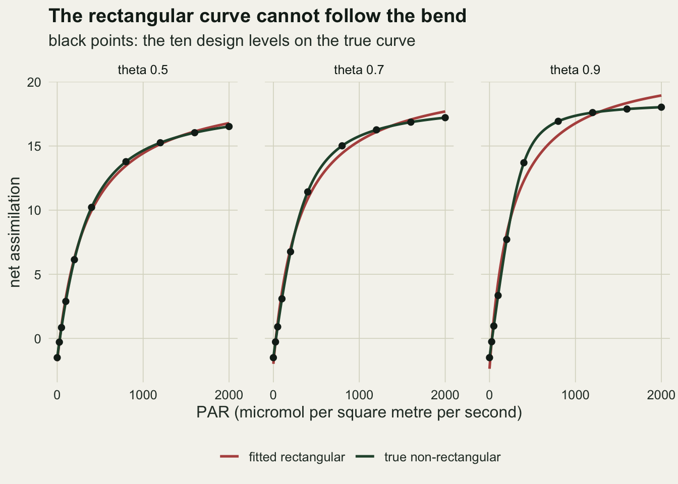
proj_long <- rbind(
  data.frame(proj_tab[, c("theta", "design")], parameter = "quantum yield",
             ratio = proj_tab$alpha_ratio),
  data.frame(proj_tab[, c("theta", "design")], parameter = "light saturated rate",
             ratio = proj_tab$pmax_ratio))
proj_long$parameter <- factor(proj_long$parameter,
                              levels = c("quantum yield", "light saturated rate"))
proj_long$design <- factor(proj_long$design, levels = names(design_list))

ggplot(proj_long, aes(theta, ratio, colour = design)) +
  geom_hline(yintercept = 1, linetype = "dashed", colour = te_body) +
  geom_line(linewidth = 0.9) +
  geom_point(size = 2.4) +
  facet_wrap(~ parameter, nrow = 1) +
  scale_colour_manual(values = c(te_gold, te_forest, te_rust), name = NULL) +
  scale_x_continuous(breaks = theta_set) +
  scale_y_continuous(breaks = seq(1, 2.2, by = 0.2)) +
  labs(x = "true curvature theta", y = "fitted / true",
       title = "A bias set by curvature and design",
       subtitle = "rectangular hyperbola fitted to the exact curve; dashed: no bias") +
  theme_datasheet() +
  theme(legend.position = "bottom")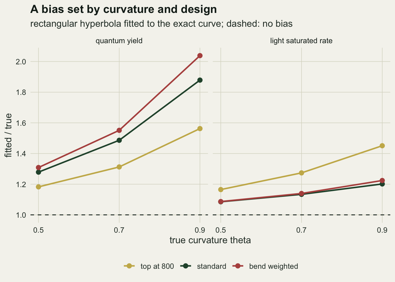
Will ten noisy points show it?
The projection says what the wrong model returns. It does not say whether anyone would notice. The size of the misfit that the data could expose is also fixed: it is the residual sum of squares of the noise-free rectangular fit, 1.59 at theta 0.7 on the standard design. Divided by the noise variance it plays the part of a noncentrality: how many noise units of evidence against the rectangular curve a curve of ten points contains on average. Whether that translates into a model choice is the part that needs simulation.
Each simulated curve adds independent normal noise to the ten true values and fits both models by least squares. The non-rectangular model is preferred when its AIC is lower by more than 2. The same comparison is repeated with the small sample correction AICc of Hurvich and Tsai, which with ten points and four or five estimated parameters (the noise variance counts) adds a heavy penalty to the larger model.
run_cell <- function(par_i, theta_k, noise_sd, n_curve) {
  mu_i <- nrh_curve(par_i, alpha_true, pmax_true, theta_k, rd_true)
  n_pt <- length(par_i)
  out <- matrix(NA_real_, n_curve, 9, dimnames = list(NULL,
    c("a_rh", "p_rh", "r_rh", "a_nr", "p_nr", "th_nr", "r_nr", "d_aic", "d_aicc")))
  for (i in seq_len(n_curve)) {
    y_obs <- mu_i + rnorm(n_pt, 0, noise_sd)
    f_rh <- fit_rh(par_i, y_obs)
    f_nr <- fit_nrh(par_i, y_obs)
    if (!is.null(f_rh)) out[i, 1:3] <- coef(f_rh)
    if (!is.null(f_nr)) out[i, 4:7] <- coef(f_nr)
    if (!is.null(f_rh) && !is.null(f_nr)) {
      aic_rh <- AIC(f_rh)
      aic_nr <- AIC(f_nr)
      out[i, "d_aic"]  <- aic_rh - aic_nr
      out[i, "d_aicc"] <- (aic_rh + 2 * 4 * 5 / (n_pt - 5)) -
                          (aic_nr + 2 * 5 * 6 / (n_pt - 6))
    }
  }
  out
}

summ_cell <- function(out) {
  ok_fit <- !is.na(out[, "d_aic"])
  th_est <- out[!is.na(out[, "th_nr"]), "th_nr"]
  c(n_ok     = sum(ok_fit),
    fail_rh  = sum(is.na(out[, "a_rh"])),
    fail_nr  = sum(is.na(out[, "a_nr"])),
    detect   = mean(out[ok_fit, "d_aic"] > 2),
    detect_c = mean(out[ok_fit, "d_aicc"] > 2),
    th_med   = median(th_est),
    th_iqr   = IQR(th_est),
    th_low   = mean(th_est < 1e-3),
    th_high  = mean(th_est > 1 - 1e-3),
    a_rh_med = median(out[, "a_rh"], na.rm = TRUE) / alpha_true,
    p_rh_med = median(out[, "p_rh"], na.rm = TRUE) / pmax_true,
    a_nr_med = median(out[, "a_nr"], na.rm = TRUE) / alpha_true,
    a_nr_iqr = IQR(out[, "a_nr"] / alpha_true, na.rm = TRUE),
    a_rh_iqr = IQR(out[, "a_rh"] / alpha_true, na.rm = TRUE),
    p_nr_iqr = IQR(out[, "p_nr"] / pmax_true, na.rm = TRUE))
}

noise_set    <- c(0.3, 0.8, 1.5)
n_grid_curve <- 300
set.seed(3014)
grid_rows <- list()
for (theta_k in theta_set) {
  for (noise_sd in noise_set) {
    s_k <- summ_cell(run_cell(design_list$standard, theta_k, noise_sd, n_grid_curve))
    grid_rows[[length(grid_rows) + 1]] <- data.frame(theta = theta_k, noise_sd = noise_sd,
                                                     t(s_k))
  }
}
grid_tab <- do.call(rbind, grid_rows)
grid_tab$ncp <- sapply(seq_len(nrow(grid_tab)), function(i)
  proj_get(grid_tab$theta[i], "standard", "rss_nf")) / grid_tab$noise_sd^2
grid_tab$se_detect <- sqrt(grid_tab$detect * (1 - grid_tab$detect) / grid_tab$n_ok)
grid_get <- function(th, s_d, col) grid_tab[grid_tab$theta == th & grid_tab$noise_sd == s_d, col]

fail_total <- sum(grid_tab$fail_rh + grid_tab$fail_nr)
n_fit_total <- 2 * n_grid_curve * nrow(grid_tab)
a_rh_gap <- max(abs(grid_tab$a_rh_med -
  sapply(grid_tab$theta, function(th) proj_get(th, "standard", "alpha_ratio"))))
knitr::kable(grid_tab[, c("theta", "noise_sd", "ncp", "detect", "detect_c",
                          "th_med", "th_iqr", "th_low", "th_high")], digits = 3,
             col.names = c("theta", "noise sd", "misfit / variance", "AIC detects",
                           "AICc detects", "theta median", "theta IQR",
"theta at 0", "theta at 1"))| theta | noise sd | misfit / variance | AIC detects | AICc detects | theta median | theta IQR | theta at 0 | theta at 1 |
|---|---|---|---|---|---|---|---|---|
| 0.5 | 0.3 | 4.997 | 0.740 | 0.220 | 0.502 | 0.214 | 0.010 | 0.000 |
| 0.5 | 0.8 | 0.703 | 0.197 | 0.033 | 0.504 | 0.653 | 0.234 | 0.000 |
| 0.5 | 1.5 | 0.200 | 0.181 | 0.020 | 0.603 | 0.877 | 0.350 | 0.050 |
| 0.7 | 0.3 | 17.715 | 0.997 | 0.783 | 0.714 | 0.124 | 0.000 | 0.000 |
| 0.7 | 0.8 | 2.491 | 0.477 | 0.080 | 0.704 | 0.295 | 0.070 | 0.007 |
| 0.7 | 1.5 | 0.709 | 0.250 | 0.027 | 0.718 | 0.510 | 0.163 | 0.103 |
| 0.9 | 0.3 | 73.793 | 1.000 | 1.000 | 0.901 | 0.039 | 0.000 | 0.000 |
| 0.9 | 0.8 | 10.377 | 0.927 | 0.520 | 0.904 | 0.116 | 0.000 | 0.027 |
| 0.9 | 1.5 | 2.952 | 0.573 | 0.127 | 0.906 | 0.214 | 0.057 | 0.147 |
At theta 0.7 and a noise standard deviation of 0.8, the middle of the three noise levels, AIC prefers the curved model in 47.7 per cent of 300 curves (Monte Carlo standard error 2.9 points). The rest of the time the data are content with the rectangular curve, and the analyst reports a quantum yield 49 per cent too high with nothing in the fit to say so. AICc detects the same curvature in 8.0 per cent of curves. With ten points the correction leaves the four parameter model rarely chosen except when the noise-free misfit is large: low noise at theta 0.7 or 0.9, or theta 0.9 at noise 0.8.
Detection is driven by the leaf as much as by the instrument. At the same noise level the rate is 0.20 at theta 0.5 and 0.93 at theta 0.9. The leaves whose quantum yield is most inflated are also the ones most likely to be caught, and the leaves with a moderate but real bias of 28 per cent are the ones that pass unnoticed. At a noise standard deviation of 1.5 even theta 0.9 is detected in only 0.57 of curves.
The noisy rectangular fits scatter around the projection, as they should. Their median quantum yield ratio sits within 0.020 of the noise-free value in every one of the 9 cells, and 2 of the 5400 fits failed to converge. That is the check that the simulation adds nothing to the bias itself.
A detection rate means little without the rate at which the same rule picks the curved model for a leaf that has no curvature. The next chunk runs the rule on a rectangular leaf, theta equal to zero, at the middle noise level.
set.seed(3017)
null_sum <- summ_cell(run_cell(design_list$standard, 0, 0.8, n_grid_curve))
null_se  <- sqrt(null_sum[["detect"]] * (1 - null_sum[["detect"]]) / null_sum[["n_ok"]])
On that rectangular leaf AIC still chose the curved model in 8.0 per cent of curves (standard error 1.6 points), and AICc in 0.7 per cent. The detection rates in the table have to be read against that floor: at theta 0.5 and the two higher noise levels AIC picked the curved model in 19.7 and 18.1 per cent of curves.
det_df <- rbind(
  data.frame(ncp = grid_tab$ncp, rate = grid_tab$detect, se = grid_tab$se_detect,
             theta = factor(grid_tab$theta), criterion = "AIC"),
  data.frame(ncp = grid_tab$ncp, rate = grid_tab$detect_c,
             se = sqrt(grid_tab$detect_c * (1 - grid_tab$detect_c) / grid_tab$n_ok),
             theta = factor(grid_tab$theta), criterion = "AICc"))

ggplot(det_df, aes(ncp, rate, shape = criterion, colour = theta)) +
  geom_errorbar(aes(ymin = pmax(rate - 2 * se, 0), ymax = pmin(rate + 2 * se, 1)),
                width = 0) +
  geom_point(size = 2.8) +
  scale_x_log10() +
  scale_colour_manual(values = c(te_gold, te_forest, te_rust), name = "theta") +
  scale_shape_manual(values = c(AIC = 16, AICc = 1), name = NULL) +
  labs(x = "noise-free misfit / noise variance (log scale)",
       y = "curves where the curved model wins",
       title = "The misfit has to be large before ten points see it",
       subtitle = "one point per curvature and noise level") +
  theme_datasheet() +
  theme(legend.position = "bottom")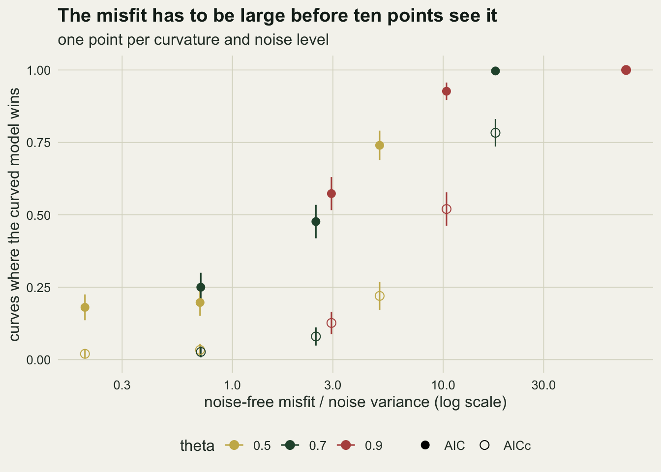
What the curved model costs
Fitting the four parameter model whenever it is affordable removes the bias: its median quantum yield ratio across the grid lies between 0.95 and 1.03. The price is mostly in theta. At theta 0.7 and noise 0.8 the interquartile range of the estimated theta is 0.30 on an interval of length one. The spread of the quantum yield is not uniformly worse: the interquartile range of its ratio to the truth is 0.30 for the curved fit and 0.30 for the biased rectangular fit in that cell, and across the grid the curved fit’s range divided by the rectangular one runs from 0.65 to 1.56, so in some cells the unbiased fit is also the tighter one.
Some fits end on a bound. At theta 0.5 and noise 1.5, 0.35 of the curved fits put theta at zero, which is the rectangular hyperbola again, and at theta 0.9 and the same noise 0.15 put it at one, the Blackman corner. A theta of exactly zero or one in a results table is therefore a statement about the data, not about the leaf, and a comparison of theta between two leaves from single ten point curves needs a difference well beyond the interquartile ranges in the table before it says anything about the leaves.
Where ten points should go
The three designs spend the same ten points. They are compared at theta 0.7 and noise 0.8, the middle of the grid, with more curves per design so that differences in detection of a few hundredths can be told from Monte Carlo error.
n_des_curve <- 800
set.seed(3015)
des_out <- lapply(design_list, function(d) run_cell(d, 0.7, 0.8, n_des_curve))
des_tab <- do.call(rbind, lapply(names(des_out), function(nm)
  data.frame(design = nm, t(summ_cell(des_out[[nm]])))))
des_tab$se_detect <- sqrt(des_tab$detect * (1 - des_tab$detect) / des_tab$n_ok)

set.seed(3016)
n_boot <- 200
des_tab$se_th_iqr <- sapply(des_out, function(out) {
  th_est <- out[!is.na(out[, "th_nr"]), "th_nr"]
  sd(replicate(n_boot, IQR(th_est[sample.int(length(th_est), replace = TRUE)])))
})
des_get <- function(dn, col) des_tab[des_tab$design == dn, col]
det_gain <- des_get("bend weighted", "detect") - des_get("standard", "detect")
det_gain_se <- sqrt(des_get("bend weighted", "se_detect")^2 + des_get("standard", "se_detect")^2)
knitr::kable(des_tab[, c("design", "detect", "se_detect", "detect_c", "th_iqr", "se_th_iqr",
                         "th_low", "a_rh_med", "a_nr_iqr", "p_nr_iqr")], digits = 3,
             col.names = c("design", "AIC detects", "MC se", "AICc detects", "theta IQR",
                           "bootstrap se", "theta at 0", "rectangular alpha ratio",
"curved alpha IQR", "curved Pmax IQR"))| design | AIC detects | MC se | AICc detects | theta IQR | bootstrap se | theta at 0 | rectangular alpha ratio | curved alpha IQR | curved Pmax IQR |
|---|---|---|---|---|---|---|---|---|---|
| top at 800 | 0.282 | 0.016 | 0.050 | 0.551 | 0.041 | 0.169 | 1.311 | 0.358 | 0.261 |
| standard | 0.500 | 0.018 | 0.102 | 0.331 | 0.016 | 0.051 | 1.484 | 0.333 | 0.102 |
| bend weighted | 0.568 | 0.018 | 0.130 | 0.276 | 0.015 | 0.034 | 1.546 | 0.304 | 0.109 |
Moving points into the bend raises the AIC detection rate from 0.50 to 0.57, a gain of 0.068 with a standard error of 0.025. It also narrows theta a little: the interquartile range is 0.331 on the standard design and 0.276 on the bend weighted one, with bootstrap standard errors of 0.016 and 0.015. Theta is still spread over a wide part of its range either way. And the same design that makes the curvature more visible makes the rectangular fit worse when it is not caught: its median quantum yield ratio is 1.55 against 1.48.
Stopping at 800 is the design to avoid. Detection falls to 0.28, theta sits at zero in 0.17 of curved fits, and even the unbiased model loses the light saturated rate: its interquartile range, as a ratio to the truth, is 0.26 against 0.10 on the standard design.
theta_df <- do.call(rbind, lapply(names(des_out), function(nm)
  data.frame(design = nm, theta_hat = des_out[[nm]][, "th_nr"])))
theta_df <- theta_df[!is.na(theta_df$theta_hat), ]
theta_df$design <- factor(theta_df$design, levels = names(design_list))

alpha_df <- do.call(rbind, lapply(names(des_out), function(nm) rbind(
  data.frame(design = nm, model = "rectangular", ratio = des_out[[nm]][, "a_rh"] / alpha_true),
  data.frame(design = nm, model = "non-rectangular", ratio = des_out[[nm]][, "a_nr"] / alpha_true))))
alpha_df <- alpha_df[!is.na(alpha_df$ratio), ]
alpha_df$design <- factor(alpha_df$design, levels = rev(names(design_list)))

p_theta <- ggplot(theta_df, aes(theta_hat)) +
  geom_histogram(breaks = seq(0, 1, by = 0.05), fill = te_forest, colour = te_paper) +
  geom_vline(xintercept = 0.7, linetype = "dashed", colour = te_rust, linewidth = 0.7) +
  facet_wrap(~ design, ncol = 1) +
  labs(x = "estimated theta", y = "curves",
       title = "Estimated theta",
       subtitle = "dashed red: true theta") +
  theme_datasheet()

p_alpha <- ggplot(alpha_df, aes(ratio, design, fill = model)) +
  geom_vline(xintercept = 1, linetype = "dashed", colour = te_body) +
  geom_boxplot(outlier.size = 0.6, outlier.alpha = 0.4, width = 0.6,
               colour = te_ink, linewidth = 0.4) +
  scale_fill_manual(values = c("rectangular" = te_rust, "non-rectangular" = te_gold),
                    name = NULL) +
  coord_cartesian(xlim = c(0, 3)) +
  labs(x = "estimated / true quantum yield", y = NULL,
       title = "Bias against spread",
       subtitle = "dashed: no bias") +
  theme_datasheet() +
  theme(legend.position = "bottom")

p_theta + p_alpha + plot_layout(widths = c(1, 1.3)) +
  plot_annotation(theme = theme_datasheet())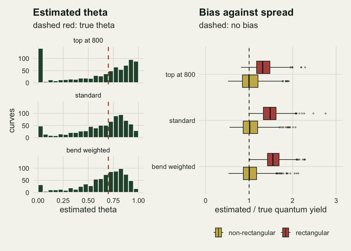
What to report
Name the model and give theta with its standard error, not only the quantum yield and light saturated rate. A rectangular hyperbola estimate of quantum yield is a projection of the leaf onto a curve with theta fixed at zero, and on the standard protocol it was 1.28 to 1.88 times the truth across the curvatures used here. Comparisons of quantum yield between species or treatments fitted this way inherit any difference in curvature as a difference in quantum yield.
Do not read a failed AIC comparison as evidence for the rectangular curve. At a moderate noise level the curved model was preferred in 47.7 per cent of the curves at theta 0.7 and in 19.7 per cent at theta 0.5, where the quantum yield was still inflated by 28 per cent. With AICc the rates are lower again. If the non-rectangular model is the physiology, fit it and carry its wider intervals.
Report the design with the parameters: the PAR levels, their order and whether dark respiration was fitted or taken from a dark reading. The projection table shows that each of these changes the number returned by the same model on the same leaf. Report fits that stopped at theta zero or one separately rather than averaging them into a species mean.
For a protocol, keep the top step at full sun and add steps between 50 and 600. That raised detection here and left the spread of the curved fit’s quantum yield and light saturated rate close to where the standard design put it. It did not make theta from one curve precise enough to compare leaves; that needs more points per curve, replicate curves per leaf, or a hierarchical fit across leaves.
Honest limits
The truth is a non-rectangular hyperbola with constant noise. Real light curves have errors that grow with the flux, points that are not independent because the leaf carries its state from one step to the next, and at the top step sometimes photoinhibition, which no hyperbola represents. A descending light sequence with incomplete acclimation adds a systematic lag that this simulation leaves out.
Only one leaf was simulated per curvature: one quantum yield, one light saturated rate and one respiration. The projection ratios depend on alpha times I relative to Pmax, so a leaf with a lower light saturated rate reaches its plateau earlier in the same design and the ratios shift. The table has to be recomputed for other parameter values; it is the method that carries over, not the numbers.
The three curvatures bracket a range rather than representing sun and shade leaves as measured types. Theta moves with carbon dioxide partial pressure, which is enough to make species and treatment comparisons of quantum yield from the rectangular fit unsafe, but the values 0.5, 0.7 and 0.9 were chosen as a sweep, not taken from a survey.
Model choice was by AIC and AICc only. A likelihood ratio test is awkward here because the rectangular curve sits on the boundary theta equal to zero, and nothing above says how such a test would behave. Bounded least squares with two starting values found the best of those starts, not a guaranteed global minimum, and the post does not measure how often a further start would have found a better fit.
References
Marshall B, Biscoe PV 1980 Journal of Experimental Botany 31(1):29-39 (10.1093/jxb/31.1.29)
Ogren E, Evans JR 1993 Planta 189(2):182-190 (10.1007/BF00195075)
Lobo FA, de Barros MP, Dalmagro HJ, Dalmolin AC, Pereira WE, de Souza EC, Vourlitis GL, Rodriguez Ortiz CE 2013 Photosynthetica 51(3):445-456 (10.1007/s11099-013-0045-y)
Hurvich CM, Tsai CL 1989 Biometrika 76(2):297-307 (10.1093/biomet/76.2.297)