---
title: "Checking a foraging analysis"
description: "Three checks for a foraging study in R: prey depletion in functional-response trials, telling type II from type III, and which currency the forager maximises."
date: "2026-06-30 14:00"
date-modified: "2026-10-08"
categories: [ecology tutorial, R, foraging, model diagnostics, behaviour]
image: thumbnail.png
image-alt: "Estimated attack rate from a disc-equation fit and a depletion-corrected fit, with the disc equation falling well short of the true value."
---
*Corrected 8 October 2026: check two said that by a density of twenty the type II and type III proportions had all but swapped places, although the curves cross just below that density; it now says they have just swapped places.*
*Corrected 1 October 2026: check three called its second currency net energy after metabolism, but the code maximises the net rate of gain, a different currency with a different prediction; the text and the printed labels now name it a net rate.*
*Updated 27 September 2026: a new part of check 2, Trials without replacement can manufacture a type III, measures how often AIC prefers a type III exponent when every predator follows type II but prey are not replaced, and how fitting the random predator equation first brings that back to the rate the arithmetic predicts.*
```{r setup}
#| code-fold: true
#| code-summary: "Setup: packages, colours and plot theme"
#| results: hide
#| message: false
#| warning: false
knitr::opts_chunk$set(echo = TRUE, message = FALSE, warning = FALSE,
                      dev = "png", dpi = 120, fig.path = "figures/",
                      fig.width = 7, fig.height = 4.4)
library(ggplot2)
theme_te <- theme_minimal(base_size = 12) +
  theme(panel.background = element_rect(fill = "#f5f4ee", colour = NA),
        plot.background  = element_rect(fill = "#f5f4ee", colour = NA),
        panel.grid.minor = element_blank(),
        plot.title = element_text(face = "bold", size = 12))
theme_set(theme_te)
col_true <- "#555555"; col_disc <- "#b5651d"; col_rog <- "#3a6b52"

## (b) type II vs III proportion eaten
propII  <- function(N) 0.9/(1 + 0.9*0.045*N)
propIII <- function(N) 0.05*N/(1 + 0.05*0.045*N^2)
Ng <- seq(1, 120, 1); peakIII <- Ng[which.max(propIII(Ng))]

## (c) currency
Gmax <- 30; k <- 0.18; g <- function(t) Gmax*(1 - exp(-k*t)); gp <- function(t) Gmax*k*exp(-k*t)
travel <- 6; mf <- 0.6
t_rate <- uniroot(function(t) gp(t) - g(t)/(t + travel), c(1e-6, 200))$root
tt_grid <- seq(0.01, 60, 0.01)
t_eff  <- tt_grid[which.max((g(tt_grid) - mf*tt_grid)/(tt_grid + travel))]
cur_diff <- 100 * abs(t_rate - t_eff)/t_rate
```
Foraging theory makes sharp predictions, and sharp predictions are easy to test against data that were not collected to test them. Three checks catch the common ways a foraging analysis goes wrong: an estimate biased by the experiment itself, two models that the data cannot separate, and a prediction that depends on a choice the analyst never stated.
## Check 1: did the prey deplete while you measured?
Holling's disc equation assumes prey density is constant through a feeding trial. It is not: as the predator eats, prey run out, so the density it experiences falls below the density you set. Fit the disc equation to trial counts anyway and the attack rate comes out too low, because the model blames slow late-trial feeding on a low attack rate rather than on missing prey. Rogers 1972 The Journal of Animal Ecology 41(2):369-383 wrote down the random predator equation, which accounts for depletion, and it is solvable in base R with `uniroot`.
```{r depletion}
a0 <- 1.0; h0 <- 0.03; Tt <- 1                          # the truth, over a trial of length 1
rogers_Ne <- function(N0) uniroot(function(Ne)          # prey eaten with depletion
  Ne - N0*(1 - exp(-a0*(Tt - h0*Ne))), c(0, N0 - 1e-9))$root

set.seed(398)                                           # six trials at each of eight densities
N0 <- rep(c(5, 10, 20, 40, 60, 80, 100, 150), each = 6)
truth <- sapply(N0, rogers_Ne)
Ne <- pmin(rbinom(length(N0), N0, truth/N0), N0)

fdisc <- nls(Ne ~ aa*N0/(1 + aa*hh*N0),                 # disc equation: density held constant
             start = list(aa = 0.5, hh = 0.02), control = nls.control(warnOnly = TRUE))
rog_pred <- function(N0, aa, hh) sapply(N0, function(n)
  uniroot(function(Ne) Ne - n*(1 - exp(-aa*(Tt - hh*Ne))), c(0, n - 1e-9))$root)
frog <- nls(Ne ~ rog_pred(N0, aa, hh),                  # random predator equation
            start = list(aa = 0.6, hh = 0.02), control = nls.control(warnOnly = TRUE))
a_disc <- coef(fdisc)["aa"]; a_rog <- coef(frog)["aa"]

c(disc_attack_rate = unname(a_disc), rogers_attack_rate = unname(a_rog), true = a0)
```
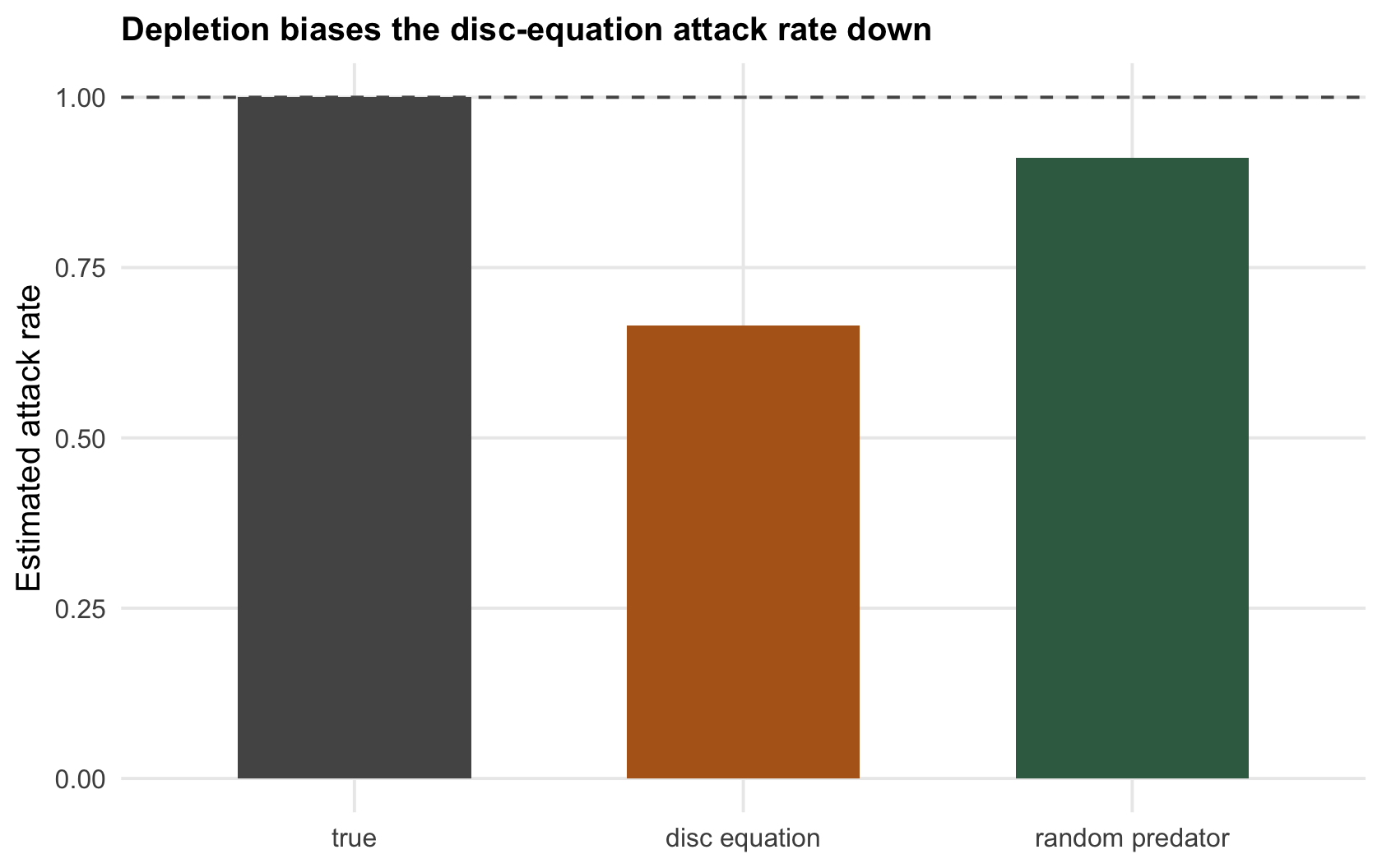
Fitting the disc equation recovers an attack rate of `r sprintf("%.2f", a_disc)`, only `r sprintf("%.0f", 100*a_disc/a0)` per cent of the true `r sprintf("%.1f", a0)`. The depletion-aware fit recovers `r sprintf("%.2f", a_rog)`, `r sprintf("%.0f", 100*a_rog/a0)` per cent. The bias is not small and it is one-directional: the disc equation fitted to trials where prey were not replaced will understate how fast the predator attacks. The check is to use the random predator equation, or to top prey up during the trial so density really is constant.
```{r fig-depletion}
#| fig-cap: "Estimated attack rate from the two fits. The disc equation, ignoring that prey deplete during a trial, lands well below the truth; the random predator equation recovers it."
#| fig-alt: "Bar chart of attack rate: a true value, a much lower disc-equation estimate, and a random-predator estimate close to the truth."
db <- data.frame(method = factor(c("true","disc equation","random predator"),
                                 levels = c("true","disc equation","random predator")),
                 a = c(a0, a_disc, a_rog))
ggplot(db, aes(method, a, fill = method)) +
  geom_col(width = 0.6) +
  geom_hline(yintercept = a0, colour = col_true, linetype = "dashed") +
  scale_fill_manual(values = c("true" = col_true, "disc equation" = col_disc, "random predator" = col_rog), guide = "none") +
  labs(x = NULL, y = "Estimated attack rate", title = "Depletion biases the disc-equation attack rate down")
```
## Check 2: can the data tell type II from type III?
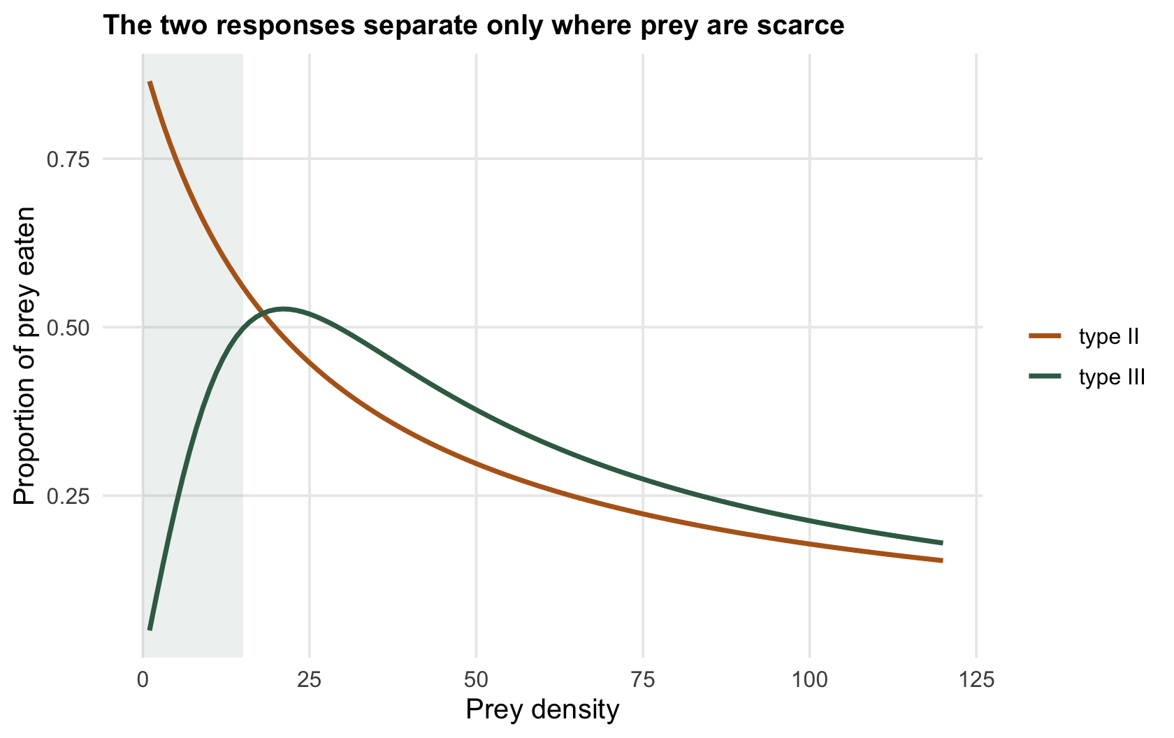
The [difference between type II and type III](../functional-responses-holling/) lives at low prey density, and so does the ability to tell them apart. The clean diagnostic is not intake but the *proportion* of prey eaten, intake divided by density. Under type II that proportion is highest at the lowest density and falls throughout. Under type III it rises to a hump and only then falls.
```{r proportion}
propII  <- function(N) 0.9/(1 + 0.9*0.045*N)             # Ne/N, type II
propIII <- function(N) 0.05*N/(1 + 0.05*0.045*N^2)       # Ne/N, type III
rbind(type_II  = round(propII(c(2, 20, 60)), 3),
      type_III = round(propIII(c(2, 20, 60)), 3))
```
At a density of 2 the two responses predict proportions of `r sprintf("%.2f", propII(2))` and `r sprintf("%.2f", propIII(2))`, a large gap. The type III proportion peaks at a density of `r peakIII` and the curves cross a little below that peak, so by a density of 20 they have just swapped places, `r sprintf("%.2f", propII(20))` against `r sprintf("%.2f", propIII(20))`, and at 60 the gap has reopened the other way, `r sprintf("%.2f", propII(60))` against `r sprintf("%.2f", propIII(60))`. If your feeding trials start at moderate densities, both curves fit and the proportion-eaten plot cannot separate them, yet they imply opposite things for whether the predator can regulate its prey. The check is to sample the low-density end deliberately, and to plot proportion eaten, not intake, where the two models actually diverge.
```{r fig-proportion}
#| fig-cap: "Proportion of prey eaten against density. Type II (ochre) falls from the start; type III (green) rises to a hump then falls. The models differ most at low density, shaded, where they also point in opposite directions; they cross near the type III hump and reopen a smaller gap above it."
#| fig-alt: "Two curves of proportion eaten against prey density; the ochre type II curve declines throughout, the green type III curve rises then declines, differing most at low density."
dp <- rbind(data.frame(N = Ng, p = propII(Ng),  type = "type II"),
            data.frame(N = Ng, p = propIII(Ng), type = "type III"))
ggplot(dp, aes(N, p, colour = type)) +
  annotate("rect", xmin = 0, xmax = 15, ymin = -Inf, ymax = Inf, fill = "#8aa29e", alpha = 0.15) +
  geom_line(linewidth = 1) +
  scale_colour_manual(values = c("type II" = col_disc, "type III" = col_rog)) +
  labs(x = "Prey density", y = "Proportion of prey eaten", colour = NULL,
       title = "The two responses differ most where prey are scarce")
```
### Trials without replacement can manufacture a type III
Sampling the low end is necessary, not sufficient. In most feeding trials the prey are not replaced, and [Check 1](#check-1-did-the-prey-deplete-while-you-measured) showed that depletion drags the disc-equation attack rate down. The same depletion bends the curve that Check 2 reads for shape: a predator that has eaten most of a small batch spends the rest of the trial searching for the few prey left, so the proportion eaten flattens at the densities where type II and type III part. That link, from depletion to a comparison of shapes, is what this part adds. Every predator below has a type II instantaneous response, that of `propII` above, with its own attack rate when predators differ. The densities are Check 1's with 80 swapped for 2, as the advice above asks, with 6 and then 20 trials per density. Each data set is fitted by binomial likelihood three ways: type II, the generalised exponent `a N^(1+q) / (1 + a h N^(1+q))` with `q > 0` (Real 1977 The American Naturalist 111(978):289-300), and the strict type III, `q = 1`. There are four kinds of trial. In two, the proportion eaten follows the disc equation exactly, as the fitted model assumes: binomial trials, and beta-binomial trials whose mean is exactly type II and only the spread is extra (a correlation of 0.12 between the fates of the prey in one trial). In the other two the prey are not replaced and each predator eats what Check 1's random predator equation says (`rog_pred` above), either the same predator every time or predators that differ, with a lognormal attack rate (standard deviation 0.6 on the log scale). For these two the chunk also fits the exponent inside the random predator equation, as an attack rate `a N^q`.
```{r false-type-three}
fr_a <- 0.9; fr_h <- 0.045                                 # propII above: the instantaneous type II
fr_N <- c(2, 5, 10, 20, 40, 60, 100, 150)                  # Check 1 densities, 80 swapped for 2
stopifnot(isTRUE(all.equal(fr_a/(1 + fr_a*fr_h*fr_N), propII(fr_N))))
fr_sdlog <- 0.6; fr_rho <- 0.12; fr_reps <- 250            # design constants, fixed before running
fr_prop <- function(N, par, q) exp(par[1])*N^q/(1 + exp(par[1] + par[2])*N^(1 + q))
rp_eat <- function(N, a, h) { Ne <- pmin(N, a*N*Tt/(1 + a*h*N))   # rog_pred as Newton steps
  for (i in 1:6) { e <- exp(-a*(Tt - h*Ne)); Ne <- Ne - (Ne - N*(1 - e))/(1 + N*a*h*e) }; Ne }
for (m in c(0.2, 1, 5))                                    # the same numbers as Check 1's solver
  stopifnot(isTRUE(all.equal(rp_eat(fr_N, m*fr_a, fr_h), rog_pred(fr_N, m*fr_a, fr_h), tolerance = 1e-5)))
rp_prop <- function(N, par, q) rp_eat(N, exp(par[1])*N^q, exp(par[2]))/N
fr_nll <- function(par, eaten, left, q_of, pf) {          # binomial likelihood, from the totals
  p <- pmin(pmax(pf(fr_N, par, q_of(par)), 1e-9), 1 - 1e-9); -sum(eaten*log(p) + left*log(1 - p)) }
q_II <- function(par) 0; q_gen <- function(par) exp(par[3]); q_III <- function(par) 1; fr_fail <- fr_calls <- 0
fr_fit <- function(starts, N, y, q_of, pf = fr_prop) { best <- NULL   # best of several starts
  eaten <- tapply(y, N, sum); left <- tapply(N - y, N, sum)          # per density, in fr_N order
  for (s in starts) { fr_calls <<- fr_calls + 1
    o <- try(optim(s, fr_nll, eaten = eaten, left = left, q_of = q_of, pf = pf,
                   control = list(maxit = 2000)), silent = TRUE)
    if (inherits(o, "try-error") || o$convergence != 0) { fr_fail <<- fr_fail + 1; next }
    if (is.null(best) || o$value < best$value) best <- o }; best }
fr_one <- function(trials, arm) {
  N <- rep(fr_N, each = trials); p2 <- fr_a/(1 + fr_a*fr_h*N)
  a_i <- fr_a*exp(if (arm == "predators differ") fr_sdlog*rnorm(length(N)) else 0)
  p <- switch(arm, "binomial" = p2,
    "beta-binomial" = rbeta(length(N), p2*(1 - fr_rho)/fr_rho, (1 - p2)*(1 - fr_rho)/fr_rho),
    rp_eat(N, a_i, fr_h)/N)                                # no replacement: Check 1's equation
  y <- rbinom(length(N), N, p)
  m2 <- fr_fit(list(log(c(fr_a, fr_h)), log(c(0.3, 0.1))), N, y, q_II)
  mq <- fr_fit(list(c(m2$par, log(1e-3)), c(m2$par, log(0.3)), log(c(0.3, 0.05, 0.5))), N, y, q_gen)
  m3 <- fr_fit(list(log(c(0.05, fr_h)), log(c(0.01, 0.02))), N, y, q_III)
  mu <- N*fr_prop(N, m2$par, 0)
  disp <- sum((y - mu)^2/(mu*(1 - mu/N)))/(length(y) - 2) # Pearson dispersion of the type II fit
  lr <- max(2*(m2$value - mq$value), 0); lr_rp <- disp_rp <- NA
  if (arm %in% c("same predator", "predators differ")) {  # the exponent inside Check 1's equation
    r2 <- fr_fit(list(m2$par, log(c(fr_a, fr_h))), N, y, q_II, rp_prop)
    rq <- fr_fit(list(c(r2$par, log(1e-3)), c(r2$par, log(0.3))), N, y, q_gen, rp_prop)
    lr_rp <- max(2*(r2$value - rq$value), 0); mu <- N*rp_prop(N, r2$par, 0)
    disp_rp <- sum((y - mu)^2/(mu*(1 - mu/N)))/(length(y) - 2) }
  c(aic = lr > 4, quasi_F = pf(lr/disp, 1, length(y) - 3, lower.tail = FALSE) < 0.05,
    strict_III = m3$value < m2$value - 1, exponent = 1 + exp(mq$par[3]), disp = disp,
    aic_rpe = lr_rp > 4, disp_rpe = disp_rp) }
fr_tab <- data.frame(arm = rep(c("binomial", "beta-binomial", "same predator", "predators differ"), each = 2), trials = c(6, 20))
set.seed(3451)
fr_runs <- Map(function(tr, arm) replicate(fr_reps, fr_one(tr, arm)), fr_tab$trials, fr_tab$arm)
fr_tab <- cbind(fr_tab, t(sapply(fr_runs, function(r) c(rowMeans(r[c("aic", "quasi_F", "strict_III", "aic_rpe"), ]),
  exponent = median(r["exponent", r["aic", ] == 1]), disp = median(r["disp", ]),
  disp_rpe = median(r["disp_rpe", ])))))
fr_cf <- function(phi) 0.5*pchisq(4/phi, 1, lower.tail = FALSE)   # the half chi-square rate
fr_tab$formula <- fr_cf(fr_tab$disp); fr_tab$formula_rpe <- fr_cf(fr_tab$disp_rpe)
fr_mcse <- sqrt(fr_tab$formula*(1 - fr_tab$formula)/fr_reps)
fr_ref <- fr_tab$arm %in% c("binomial", "beta-binomial")  # guards: the fitter, and the closed form
stopifnot(fr_tab$aic[fr_tab$arm == "binomial"] < 0.08, abs(fr_tab$aic - fr_tab$formula)[fr_ref] < 4*fr_mcse[fr_ref])
fr_r <- function(arm, trials, col) fr_tab[fr_tab$arm == arm & fr_tab$trials == trials, col]
print(cbind(fr_tab[, 1:2], round(fr_tab[, c("aic", "quasi_F", "disp", "formula", "aic_rpe", "formula_rpe")], 3)), row.names = FALSE)
fr_bend <- rbind(density = fr_N[1:4], disc = propII(fr_N[1:4]), random_predator = rog_pred(fr_N[1:4], fr_a, fr_h)/fr_N[1:4])
round(fr_bend, 3)
```
With binomial trials the generalised exponent beats type II by more than 2 AIC units in `r sprintf("%.3f", fr_r("binomial", 6, "aic"))` and `r sprintf("%.3f", fr_r("binomial", 20, "aic"))` of data sets, at 6 and 20 trials per density, and with beta-binomial trials in `r sprintf("%.3f", fr_r("beta-binomial", 6, "aic"))` and `r sprintf("%.3f", fr_r("beta-binomial", 20, "aic"))`. Without replacement it wins in `r sprintf("%.3f", fr_r("same predator", 6, "aic"))` and `r sprintf("%.3f", fr_r("same predator", 20, "aic"))` of data sets when the predator is always the same, and in `r sprintf("%.3f", fr_r("predators differ", 6, "aic"))` and `r sprintf("%.3f", fr_r("predators differ", 20, "aic"))` when predators differ. Each rate comes from `r fr_reps` data sets, so its Monte Carlo standard error is about `r sprintf("%.3f", sqrt(0.2*0.8/fr_reps))` near a rate of 0.2 and `r sprintf("%.3f", sqrt(0.02*0.98/fr_reps))` near 0.02. The strict type III is not what wins: it beats type II in at most `r sprintf("%.3f", max(fr_tab$strict_III))` of the data sets in any cell, and when the generalised exponent does win, its median fitted exponent `1 + q` is between `r sprintf("%.2f", min(fr_tab$exponent, na.rm = TRUE))` and `r sprintf("%.2f", max(fr_tab$exponent, na.rm = TRUE))`, much nearer 1 than 2. Of the `r sprintf("%d", fr_calls)` optimiser runs, `r if (fr_fail == 0) "none" else sprintf("%d", fr_fail)` stopped without converging.
Part of this is arithmetic. With one extra parameter, dAIC > 2 is a likelihood-ratio statistic above 4. Under type II the extra exponent sits on its boundary, `q = 0`, so the statistic is zero in about half of data sets and chi-square on one degree of freedom in the rest. When the extra spread leaves the mean curve exactly type II, as in the binomial and beta-binomial trials, overdispersion by a factor `phi` (the Pearson dispersion of the type II fit) stretches the statistic by `phi`, and the expected rate is `0.5 P(chi2_1 > 4 / phi)`, the `formula` column: `r sprintf("%.3f", fr_r("binomial", 6, "formula"))` and `r sprintf("%.3f", fr_r("binomial", 20, "formula"))` for binomial trials, `r sprintf("%.3f", fr_r("beta-binomial", 6, "formula"))` and `r sprintf("%.3f", fr_r("beta-binomial", 20, "formula"))` for beta-binomial trials at dispersions of `r sprintf("%.1f", fr_r("beta-binomial", 6, "disp"))` and `r sprintf("%.1f", fr_r("beta-binomial", 20, "disp"))`. The simulation reproduces both, every one of these four rates lying within `r sprintf("%.1f", max((abs(fr_tab$aic - fr_tab$formula)/fr_mcse)[fr_ref]))` Monte Carlo standard errors of its formula. For the beta-binomial trials the match is only approximate: their dispersion grows with density, as `1 + (N - 1) * 0.12`, and one `phi` stands in for all of it.
Depletion is not spread, and the formula does not see it. With the same predator every time the dispersion is `r sprintf("%.2f", fr_r("same predator", 6, "disp"))` and `r sprintf("%.2f", fr_r("same predator", 20, "disp"))` and the formula gives `r sprintf("%.3f", fr_r("same predator", 20, "formula"))`, yet at 20 trials per density the exponent wins `r sprintf("%.1f", fr_r("same predator", 20, "aic")/fr_r("same predator", 20, "formula"))` times as often. At 6 trials the excess is smaller, `r sprintf("%.1f", (fr_r("same predator", 6, "aic") - fr_r("same predator", 6, "formula"))/fr_mcse[fr_tab$arm == "same predator" & fr_tab$trials == 6])` Monte Carlo standard errors in this run: the rate grows with the number of trials, as it does when the bend is in the mean. The second table shows the bend: between densities of 2 and 20 the disc equation's proportion eaten falls from `r sprintf("%.2f", fr_bend["disc", 1])` to `r sprintf("%.2f", fr_bend["disc", 4])`, one predator eating without replacement from `r sprintf("%.2f", fr_bend["random_predator", 1])` to `r sprintf("%.2f", fr_bend["random_predator", 4])`. A flat start is what an exponent above 1 draws, and the more trials there are, the more often the likelihood takes it. Predators that differ add spread on top, dispersions of `r sprintf("%.2f", fr_r("predators differ", 6, "disp"))` and `r sprintf("%.2f", fr_r("predators differ", 20, "disp"))`, which lifts the AIC rate further. Scaling by the dispersion is no repair for the bend: dividing the deviance difference by the Pearson dispersion and referring it to `F(1, n - 3)` cuts the beta-binomial rates to `r sprintf("%.3f", fr_r("beta-binomial", 6, "quasi_F"))` and `r sprintf("%.3f", fr_r("beta-binomial", 20, "quasi_F"))`, but leaves `r sprintf("%.3f", fr_r("same predator", 6, "quasi_F"))` and `r sprintf("%.3f", fr_r("same predator", 20, "quasi_F"))` with the same predator and `r sprintf("%.3f", fr_r("predators differ", 6, "quasi_F"))` and `r sprintf("%.3f", fr_r("predators differ", 20, "quasi_F"))` when predators differ, against `r sprintf("%.3f", fr_r("binomial", 6, "quasi_F"))` and `r sprintf("%.3f", fr_r("binomial", 20, "quasi_F"))` with binomial trials.
The check, then: when prey were not replaced, fit the random predator equation first and compare shapes inside it. With the exponent in its attack rate, the exponent beats the plain equation in `r sprintf("%.3f", fr_r("same predator", 6, "aic_rpe"))` and `r sprintf("%.3f", fr_r("same predator", 20, "aic_rpe"))` of data sets with the same predator and `r sprintf("%.3f", fr_r("predators differ", 6, "aic_rpe"))` and `r sprintf("%.3f", fr_r("predators differ", 20, "aic_rpe"))` when predators differ, each within `r sprintf("%.1f", max(abs(fr_tab$aic_rpe - fr_tab$formula_rpe)/sqrt(fr_tab$formula_rpe*(1 - fr_tab$formula_rpe)/fr_reps), na.rm = TRUE))` Monte Carlo standard errors of what the formula gives at the dispersion of that fit (`formula_rpe`). Report that dispersion before comparing shapes. Variation between units that a binomial likelihood counts as independent information also leaves an exponent's interval too narrow in [Density or frequency transmission in enclosures](../density-or-frequency-dependent-transmission/), and extra spread bends a flat trend in [Overdispersion, year noise and a wiggly GAM trend](../overdispersion-and-a-wiggly-trend/).
## Check 3: which currency is the forager counting?
The [marginal value theorem](../the-marginal-value-theorem/) and the diet model both assume the forager maximises the long-run rate of energy intake. That is a choice, not a fact. An animal saving for a lean season may maximise its net rate of gain after paying its own foraging metabolism; one at risk of predation may minimise exposure time. Different currencies give different predictions from the same gain curve.
```{r currency}
g <- function(t) 30*(1 - exp(-0.18*t)); gp <- function(t) 30*0.18*exp(-0.18*t)
t_rate <- uniroot(function(t) gp(t) - g(t)/(t + 6), c(1e-6, 200))$root      # maximise rate
tt <- seq(0.01, 60, 0.01)
t_eff  <- tt[which.max((g(tt) - 0.6*tt)/(tt + 6))]                          # net of metabolism
round(c(gross_rate_currency = t_rate, net_rate_currency = t_eff), 2)
```
A forager maximising its gross rate of intake leaves the patch at `r sprintf("%.1f", t_rate)`; one maximising its net rate, after paying its own metabolism while in the patch, leaves at `r sprintf("%.1f", t_eff)`, a `r sprintf("%.0f", cur_diff)` per cent difference in predicted residence, with no change to the environment. When observed behaviour misses a rate-maximising prediction, the first question is not whether the theory is wrong but whether you guessed the currency (Pyke 1984 Annual Review of Ecology and Systematics 15(1):523-575). State the currency, and where you can, test more than one.
## Deviations are data
Foraging theory is a set of predictions about an optimiser, and animals are not optimisers so much as satisficers working with partial information and real risk. That is why these models earn their keep even when animals depart from them: a clean prediction turns every departure into a measurement. A predator that eats a poor prey it should ignore is telling you about recognition error or nutrient needs; a forager that stays in a patch too long is telling you about uncertainty or safety. Run the three checks so the numbers are sound, then read the residuals as biology, not as failure.
## References
- Holling CS 1959. The Canadian Entomologist 91(7):385-398 (10.4039/Ent91385-7).
- Pyke GH 1984. Annual Review of Ecology and Systematics 15(1):523-575 (10.1146/annurev.es.15.110184.002515).
- Real LA 1977. The American Naturalist 111(978):289-300 (10.1086/283161).
- Rogers D 1972. The Journal of Animal Ecology 41(2):369-383 (10.2307/3474).
## Related tutorials
- [Functional responses in R](../functional-responses-holling/)
- [The marginal value theorem](../the-marginal-value-theorem/)
- [Diet choice and the zero-one rule](../diet-choice-and-the-zero-one-rule/)
- [Nonlinear regression with nls](../nonlinear-regression-with-nls/)