---
title: "Functional responses in R"
description: "Holling's functional responses in R: the type I, II and III curves, fitting the disc equation with nls, and why handling time sets a ceiling on mean intake."
date: "2026-06-30 13:00"
date-modified: "2026-10-07"
categories: [ecology tutorial, R, foraging, species interactions, predation]
image: thumbnail.png
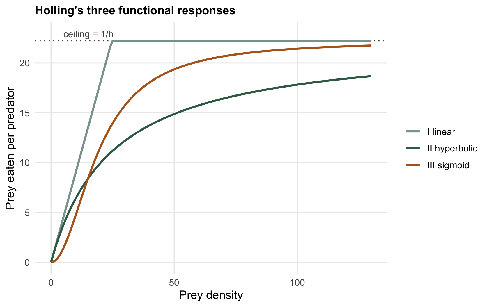
image-alt: "Three functional response curves rising from the origin against prey density: a straight climb that stops dead at a dotted ceiling near 22 prey eaten per predator, an S-shaped curve that comes within a fraction of that ceiling at the right edge, and a hyperbola still climbing about a sixth below it."
---
*Corrected 7 October 2026: the post said intake cannot exceed the fitted ceiling of one over the handling time, however much prey there is; that ceiling is an estimate for mean intake, not a cap on single trials, some of which lie above it here, and the text, the description and the caption and plot title of the fitted-curve figure now say so.*
```{r setup}
#| code-fold: true
#| code-summary: "Setup: packages, colours and plot theme"
#| results: hide
#| message: false
#| warning: false
knitr::opts_chunk$set(echo = TRUE, message = FALSE, warning = FALSE,
                      dev = "png", dpi = 120, fig.path = "figures/",
                      fig.width = 7, fig.height = 4.4)
library(ggplot2)
theme_te <- theme_minimal(base_size = 12) +
  theme(panel.background = element_rect(fill = "#f5f4ee", colour = NA),
        plot.background  = element_rect(fill = "#f5f4ee", colour = NA),
        panel.grid.minor = element_blank(),
        plot.title = element_text(face = "bold", size = 12))
theme_set(theme_te)
col1 <- "#8aa29e"; col2 <- "#3a6b52"; col3 <- "#b5651d"; col_ref <- "#555555"

holl2 <- function(N, a, h, T = 1) a*N*T / (1 + a*h*N)
holl3 <- function(N, a, h, T = 1) a*N^2*T / (1 + a*h*N^2)

set.seed(395)
a0 <- 0.9; h0 <- 0.045
N  <- rep(c(2, 5, 10, 20, 40, 60, 80, 120), each = 5)
Ne <- rpois(length(N), holl2(N, a0, h0))
fit2 <- nls(Ne ~ aa*N/(1 + aa*hh*N), start = list(aa = 0.5, hh = 0.05))
cf <- coef(fit2); a_hat <- cf["aa"]; h_hat <- cf["hh"]; ceiling_rate <- 1/h_hat
int120 <- holl2(120, a_hat, h_hat); pct120 <- 100 * int120 / ceiling_rate
```
How fast a predator eats depends on how much prey there is, but not in a straight line. Double the prey and a predator does not eat twice as much, because catching prey takes time and eating them takes more. The curve relating prey density to intake rate is the functional response, and Holling 1959 The Canadian Entomologist 91(7):385-398 sorted it into three shapes that still organise the subject.
## Three shapes
**Type I** is the straight line: intake rises in proportion to prey density, then stops dead at a ceiling. It fits filter feeders and little else, because it assumes handling prey costs no time until, abruptly, it does.
**Type II** is the workhorse. Intake rises steeply at low density and bends over to a plateau, because every prey item caught must be handled, and handling time eats into searching time. Holling's disc equation captures it with two parameters, an attack rate `a` and a handling time `h`:
$$N_e = \frac{a\,N\,T}{1 + a\,h\,N}.$$
**Type III** is S-shaped: intake accelerates at low prey density before bending over. The acceleration can come from predators learning to find a prey type only once it is common, or switching to whatever is abundant. That low-density dip matters out of proportion to its size, as the last section explains.
```{r curves}
holl2 <- function(N, a, h, T = 1) a*N*T / (1 + a*h*N)
holl3 <- function(N, a, h, T = 1) a*N^2*T / (1 + a*h*N^2)
Ngrid <- seq(0, 130, 1)
c(type2_at_40 = holl2(40, 0.9, 0.045), type3_at_40 = holl3(40, 0.06, 0.045))
```
```{r fig-types}
#| fig-cap: "The three functional responses. Type I (grey) is linear to a ceiling; type II (green) saturates smoothly; type III (ochre) is S-shaped, with a low-density region where intake accelerates."
#| fig-alt: "Three curves of intake against prey density: a straight grey line to a plateau, a green hyperbola bending to a plateau, and an ochre S-shaped curve reaching the same plateau."
capk <- 1/0.045
d <- rbind(
  data.frame(N = Ngrid, y = pmin(0.9 * Ngrid, capk), type = "I linear"),
  data.frame(N = Ngrid, y = holl2(Ngrid, 0.9, 0.045),  type = "II hyperbolic"),
  data.frame(N = Ngrid, y = holl3(Ngrid, 0.06, 0.045), type = "III sigmoid"))
ggplot(d, aes(N, y, colour = type)) +
  geom_hline(yintercept = capk, colour = col_ref, linetype = "dotted") +
  geom_line(linewidth = 1) +
  annotate("text", x = 5, y = capk + 0.7, label = "ceiling = 1/h", hjust = 0, colour = col_ref, size = 3.4) +
  scale_colour_manual(values = c("I linear" = col1, "II hyperbolic" = col2, "III sigmoid" = col3)) +
  labs(x = "Prey density", y = "Prey eaten per predator", colour = NULL,
       title = "Holling's three functional responses")
```
## Fitting a type II curve
Given feeding-trial counts, the disc equation fits straight away with `nls`. Over a total time `T` of one, the number eaten per predator is `a N / (1 + a h N)`.
```{r fit}
set.seed(395)
N  <- rep(c(2, 5, 10, 20, 40, 60, 80, 120), each = 5)
Ne <- rpois(length(N), 0.9 * N / (1 + 0.9 * 0.045 * N))     # type II truth
fit2 <- nls(Ne ~ aa * N / (1 + aa * hh * N), start = list(aa = 0.5, hh = 0.05))
round(coef(fit2), 4)
```
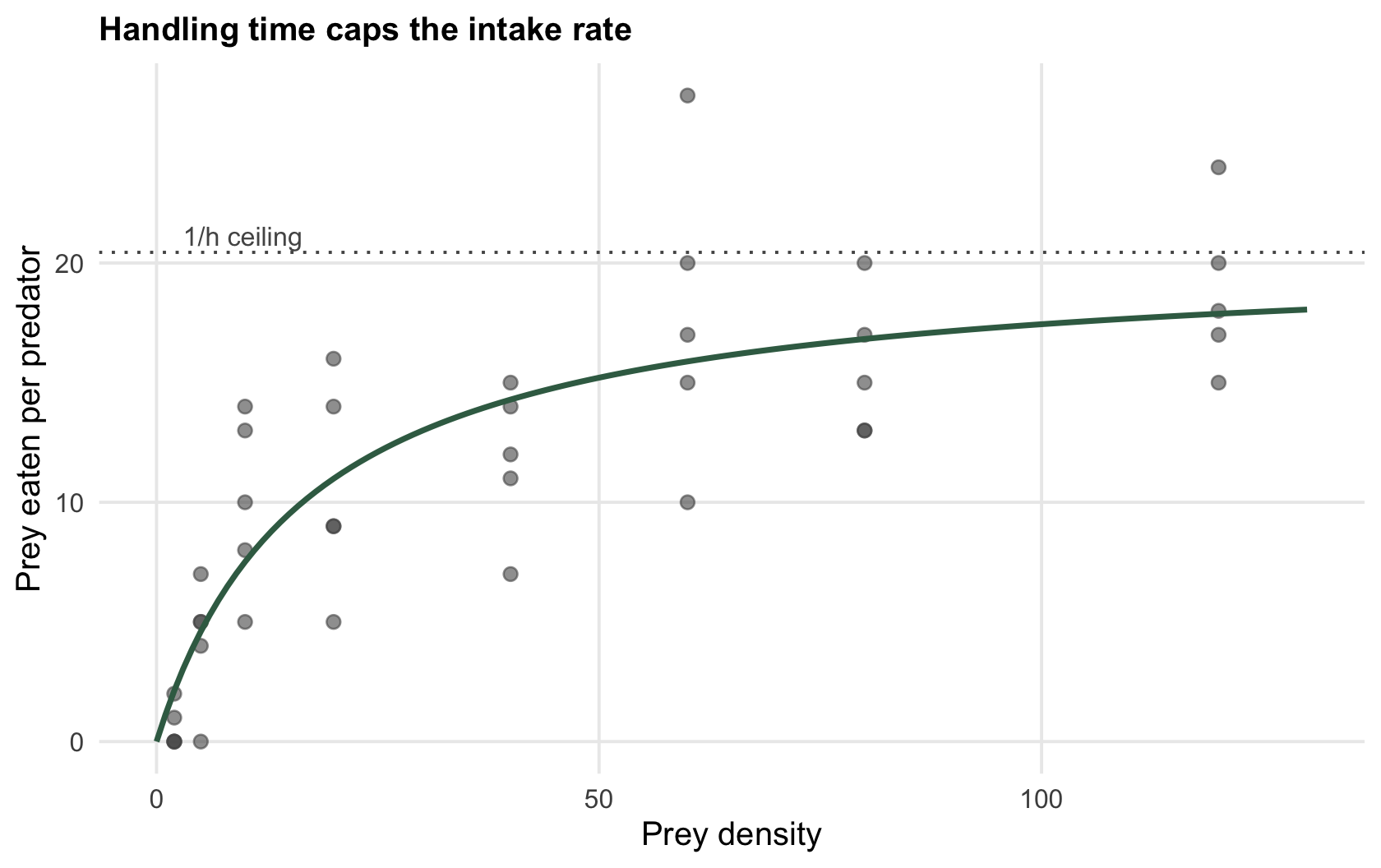
The fit returns an attack rate of `r sprintf("%.2f", a_hat)` and a handling time of `r sprintf("%.4f", h_hat)`. That handling time is the more useful number, because it sets a ceiling. As prey density climbs, the fitted mean intake levels off towards `r sprintf("%.1f", ceiling_rate)` prey per unit time, the reciprocal of the estimated handling time, and never passes it however much prey there is. That ceiling is an estimate for mean intake, not a cap on single trials: counts scatter around the curve, and some of these trials lie above it. At a density of 120 the predator is already taking `r sprintf("%.1f", int120)`, which is `r sprintf("%.0f", pct120)` per cent of that ceiling.
```{r fig-fit}
#| fig-cap: "A type II fit to feeding-trial counts. The fitted curve levels off towards one over the estimated handling time (dotted), a ceiling on mean intake; single trials scatter around the curve, and some lie above that line."
#| fig-alt: "Scatter of prey eaten against prey density with a saturating fitted curve levelling off at a dotted ceiling line."
pf <- data.frame(N = Ngrid, y = holl2(Ngrid, a_hat, h_hat))
ggplot(data.frame(N, Ne), aes(N, Ne)) +
  geom_hline(yintercept = ceiling_rate, colour = col_ref, linetype = "dotted") +
  geom_point(colour = col_ref, size = 2, alpha = 0.6) +
  geom_line(data = pf, aes(N, y), colour = col2, linewidth = 1) +
  annotate("text", x = 3, y = ceiling_rate + 0.7, label = "1/h ceiling", hjust = 0, colour = col_ref, size = 3.4) +
  labs(x = "Prey density", y = "Prey eaten per predator", title = "Handling time caps the mean intake rate")
```
## Why the shape matters for stability
The difference between type II and type III is not cosmetic. Divide intake by prey density to get the *per-capita* predation risk a prey individual faces. Under a type II response that risk is highest when prey are rare and falls as prey become common: the predator is easily satiated, so being scarce is dangerous. That is destabilising; it can drive prey to local extinction. Under a type III response the risk is low when prey are rare, because the predator ignores or cannot find a scarce prey type, giving prey a low-density refuge that can stabilise the interaction (see [stability and complexity in food webs](../stability-and-complexity-in-food-webs/)).
So the interesting part of a functional response is exactly the part that is hardest to measure: the behaviour at low prey density. Two curves that look identical at the densities you sampled can imply opposite dynamics. The [checking post](../checking-a-foraging-analysis/) returns to this, along with the trap that prey deplete while you are measuring. The two posts before this one leave the predator's plate and ask how a forager should spend its time: [how long to stay in a patch](../the-marginal-value-theorem/), and [which prey to bother with at all](../diet-choice-and-the-zero-one-rule/).
## References
- Holling CS 1959. The Canadian Entomologist 91(7):385-398 (10.4039/Ent91385-7).
- Pyke GH 1984. Annual Review of Ecology and Systematics 15(1):523-575 (10.1146/annurev.es.15.110184.002515).
- Rogers D 1972. The Journal of Animal Ecology 41(2):369-383 (10.2307/3474).
## Related tutorials
- [The marginal value theorem](../the-marginal-value-theorem/)
- [Diet choice and the zero-one rule](../diet-choice-and-the-zero-one-rule/)
- [Checking a foraging analysis](../checking-a-foraging-analysis/)
- [Stability and complexity in food webs](../stability-and-complexity-in-food-webs/)