stable <- function(M) max(Re(eigen(M, only.values = TRUE)$values)) < 0Stability and complexity in food webs
R
food webs
stability
community ecology
ecology tutorial
May’s stability criterion in R: build community matrices, find when large complex systems lose stability, and why predator-prey structure moves the boundary.
Corrected 15 October 2026: the post described its predator-prey webs only as antagonistic pairs; it now says that the code always makes the lower-numbered species of a pair the predator, a fixed feeding order, while the threshold formula it quotes is for webs in which the predator of each pair is chosen at random.
Corrected 7 October 2026: the closing section said this post used the niche model idea of a web; its webs have links placed at random at a given size and connectance, without the structure of the niche model, and the sentence now says so.
For decades ecologists believed that complexity begets stability: more species and more links should make a community harder to destabilise. In 1972 Robert May showed the opposite in a few lines of linear algebra. If you build a large system with random interactions, there is a sharp threshold in interaction strength beyond which it is almost certain to be unstable, and the threshold gets stricter as the system grows. This post reproduces May’s result in R, then follows Allesina and Tang’s 2012 refinement: the sign structure of the interactions, not just their number, decides where the threshold sits, and predator-prey webs sit far on the stable side of a random one.
The community matrix
Near an equilibrium, a community is summarised by its Jacobian, the community matrix M. Entry M[i, j] is the effect of a small change in species j on the growth rate of species i. The equilibrium is locally stable when every eigenvalue of M has a negative real part, so any small perturbation decays. One number decides it: the largest real part across all eigenvalues.
May’s construction is deliberately blunt. Put self-regulation on the diagonal, -d, so each species alone returns to equilibrium. Off the diagonal, let a fraction C of the entries be non-zero (the connectance), each an independent draw from a normal distribution with standard deviation sigma (the typical interaction strength). Nothing about who eats whom, just random couplings of a given density and strength.
mat_random <- function(S, C, sigma, d = 1) {
  E <- matrix(rnorm(S * S), S, S) * (matrix(runif(S * S), S, S) < C)
  diag(E) <- 0
  -d * diag(S) + sigma * E
}
The threshold
May’s result is that a large random system is almost surely stable when sigma * sqrt(S * C) < d, and almost surely unstable above it. Rearranged, the critical interaction strength is d / sqrt(S * C): larger systems (more species S, denser webs C) tolerate weaker interactions before they tip. Take 50 species at connectance 0.2 and unit self-regulation.
S <- 50; C <- 0.20; d <- 1
sigma_crit <- d / sqrt(S * C)
round(sigma_crit, 3)
[1] 0.316The predicted threshold is 0.316. Sweep the interaction strength across it and count how often a freshly built system is stable.
set.seed(2024)
sigmas <- seq(0.15, 0.55, by = 0.05)
frac_stable <- sapply(sigmas, function(s)
  mean(replicate(300, stable(mat_random(S, C, s, d)))))
data.frame(sigma = sigmas, stable = frac_stable)
sigma stable
1 0.15 1.000000000
2 0.20 1.000000000
3 0.25 1.000000000
4 0.30 0.896666667
5 0.35 0.456666667
6 0.40 0.063333333
7 0.45 0.006666667
8 0.50 0.000000000
9 0.55 0.000000000library(ggplot2)
df <- data.frame(sigma = sigmas, stable = frac_stable)
ggplot(df, aes(sigma, stable)) +
geom_vline(xintercept = sigma_crit, linetype = "dashed", colour = "grey55") +
geom_line(colour = "#3d6cb0", linewidth = 0.8) +
geom_point(colour = "#3d6cb0", size = 2) +
annotate("text", x = sigma_crit + 0.005, y = 0.9, label = "May threshold",
hjust = 0, size = 3.4, colour = "grey35") +
labs(x = "Interaction strength (sigma)", y = "Fraction stable") +
theme_minimal(base_size = 12) +
theme(panel.grid.minor = element_blank(),
plot.background = element_rect(fill = "#f5f4ee", colour = NA),
panel.background = element_rect(fill = "#f5f4ee", colour = NA))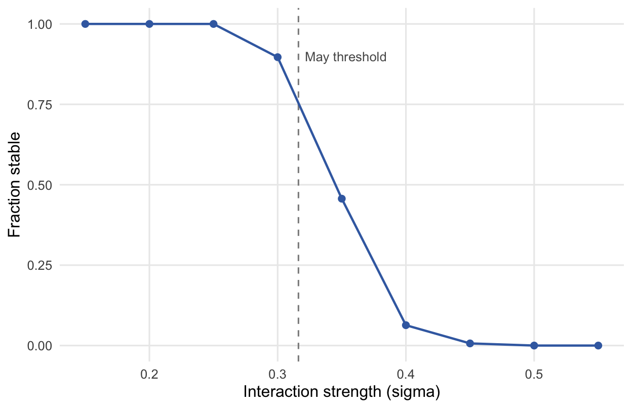
The collapse lands where May said it would. At sigma = 0.30, just below the threshold, 90% of systems are stable; at 0.40, well above it, only 6%. The transition is sharp because it is driven by the rightmost eigenvalue of a large random matrix, which for these matrices sits close to sigma * sqrt(S * C) - d. When that crosses zero, stability flips.
set.seed(11)
big <- sapply(c(0.2, 0.3, 0.4), function(s) {
  M <- mat_random(200, C, s, d)
  c(sigma = s,
    observed  = max(Re(eigen(M, only.values = TRUE)$values)),
    predicted = s * sqrt(200 * C) - d)
})
round(t(big), 3)
sigma observed predicted
[1,] 0.2 0.186 0.265
[2,] 0.3 1.009 0.897
[3,] 0.4 1.659 1.530For a 200-species system the observed rightmost eigenvalue lands within about 0.13 of the prediction at each interaction strength, below it at the weakest and above it at the other two. That is close enough to show the theory is a statement about where the eigenvalue spectrum ends rather than a fitted curve, and far enough to show that 200 species is still a finite system.
Sign structure changes everything
May’s matrix has no ecology in it: an interaction between two species is two independent random numbers. Real interactions come in pairs with meaning. In a predator-prey link the effect of prey on predator is positive and the effect of predator on prey is negative. Allesina and Tang asked what that pairing does to stability, and the answer is a lot. Build the same kind of matrix, but make every interacting pair antagonistic: one direction positive, the other negative. For simplicity the code below always makes the lower-numbered species of a pair the predator, a fixed feeding order, whereas the threshold formula used further down is for webs in which the predator of each pair is chosen at random.
mat_predprey <- function(S, C, sigma, d = 1) {
  E <- matrix(0, S, S)
  for (i in 1:(S - 1)) for (j in (i + 1):S) if (runif(1) < C) {
    E[i, j] <-  abs(rnorm(1))       # prey j raises predator i
    E[j, i] <- -abs(rnorm(1))       # predator i lowers prey j
  }
  -d * diag(S) + sigma * E
}
The pairing creates a negative correlation between the two directions of each link, and that correlation is what moves the boundary. Measure it, and compare the two constructions across a much wider range of interaction strength.
# reciprocal correlation of the two directions of each link
set.seed(5)
rho <- mean(replicate(200, {
  E <- matrix(0, S, S)
  for (i in 1:(S - 1)) for (j in (i + 1):S) if (runif(1) < C) {
    E[i, j] <- abs(rnorm(1)); E[j, i] <- -abs(rnorm(1)) }
  k <- which(E != 0 & t(E) != 0)
  mean(E[k] * t(E)[k]) / mean(E[E != 0]^2)
}))

set.seed(2024)
sig_wide <- seq(0.3, 1.1, by = 0.1)
frac_pp <- sapply(sig_wide, function(s)
  mean(replicate(300, stable(mat_predprey(S, C, s, d)))))

c(reciprocal_corr = round(rho, 3),
  predator_prey_threshold = round(d / (sqrt(S * C) * (1 + rho)), 3))
reciprocal_corr predator_prey_threshold
-0.635 0.866 The reciprocal correlation is -0.635, close to the theoretical -2/pi for opposite-signed half-normal pairs. Allesina and Tang show the predator-prey threshold is May’s, divided by 1 + rho. With this correlation that is 0.866, about 2.7 times the random threshold of 0.316.
comp <- rbind(
  data.frame(sigma = sigmas,   stable = frac_stable, type = "random"),
  data.frame(sigma = sig_wide, stable = frac_pp,     type = "predator-prey")
)

ggplot(comp, aes(sigma, stable, colour = type)) +
  geom_line(linewidth = 0.8) +
  geom_point(size = 1.8) +
  scale_colour_manual(values = c("random" = "#c1523f",
                                 "predator-prey" = "#4c9f70")) +
  labs(x = "Interaction strength (sigma)", y = "Fraction stable", colour = NULL) +
  theme_minimal(base_size = 12) +
  theme(panel.grid.minor = element_blank(),
        legend.position = "top",
        plot.background = element_rect(fill = "#f5f4ee", colour = NA),
        panel.background = element_rect(fill = "#f5f4ee", colour = NA))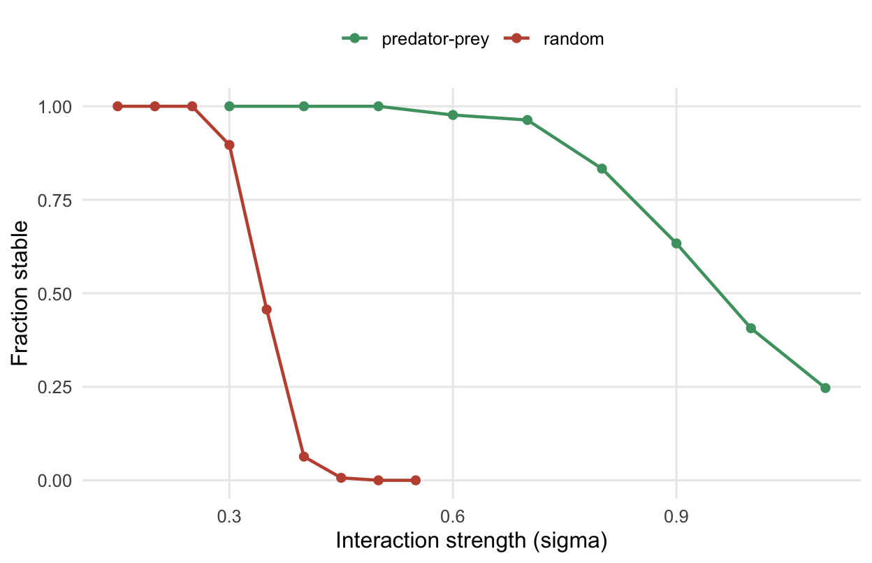
At an interaction strength of 0.40, random systems are almost all unstable (6% stable) while predator-prey systems are still entirely stable (100%). The predator-prey webs stay majority-stable out to about sigma = 0.9. Complexity still destabilises, exactly as May proved; but antagonistic pairing, which is what a food web is made of, buys a large amount of headroom that a random graph does not have.
What this does and does not say
Two cautions keep this honest. This is local stability of a linearised system with random coefficients, not the dynamics of a real, parameterised web: the interaction strengths here are arbitrary draws, not measured rates, and a locally stable equilibrium can still sit in a community that never reaches it. And the whole calculation rests on the self-regulation term d, the diagonal. It sets the scale that sigma * sqrt(S * C) is compared against, yet it is the parameter field ecologists almost never measure. The next post makes that dependence concrete: hold a web fixed and watch the stability verdict flip as the assumed self-regulation changes.
Where to go next
This post placed links at random in webs of a given size and connectance, without the structure of the niche model, which starts from the same two numbers. The checking post shows how sensitive the stability verdict is to the assumptions made here. For stability estimated from real time series rather than a random matrix, see stability from a MAR(1) model.
References
May RM 1972 Nature 238(5364):413-414 (10.1038/238413a0)
Allesina S, Tang S 2012 Nature 483(7388):205-208 (10.1038/nature10832)
McCann KS 2000 Nature 405(6783):228-233 (10.1038/35012234)
Cohen JE, Newman CM 1985 Journal of Theoretical Biology 113(1):153-156 (10.1016/S0022-5193(85)80081-3)