library(ggplot2)

te_paper  <- "#f5f4ee"
te_ink    <- "#16241d"
te_body   <- "#2c3a31"
te_forest <- "#275139"
te_rust   <- "#b5534e"
te_gold   <- "#c9b458"
te_line   <- "#dad9ca"

theme_datasheet <- function() {
  theme_minimal(base_size = 12) +
    theme(plot.background  = element_rect(fill = te_paper, colour = NA),
          panel.background = element_rect(fill = te_paper, colour = NA),
          panel.grid.major = element_line(colour = te_line, linewidth = 0.3),
          panel.grid.minor = element_blank(),
          text             = element_text(colour = te_body),
          plot.title       = element_text(colour = te_ink, face = "bold"),
          plot.subtitle    = element_text(colour = te_body),
          axis.text        = element_text(colour = te_body))
}

escape_prob <- function(pp, att, clump) {
  if (is.infinite(clump)) exp(-att * pp) else (1 + att * pp / clump)^(-clump)
}

hp_step <- function(state, lam, att, clump) {
  hh <- state[1]; pp <- state[2]
  ee <- escape_prob(pp, att, clump)
  c(lam * hh * ee, hh * (1 - ee))
}Aggregation and host parasitoid stability
R
population dynamics
host-parasitoid
stability
ecology tutorial
Why the Nicholson-Bailey host parasitoid equilibrium is unstable at every parameter: eigenvalue modulus in R, and the aggregation threshold that stabilises it.
A univoltine leaf miner and the wasp that attacks it are counted at forty patches once a year, at the end of the larval period, for twenty generations. Parasitism runs at roughly half of the mined leaves in most years. The mine counts swing by a factor of ten between consecutive generations, and the swings are getting wider rather than narrower. The question a manager asks is whether the pair will settle by itself, and if not, what would have to be true of the wasp for it to settle.
The oldest model of that pair is a pair of difference equations, one per generation, with no time in between: hosts are laid, wasps search, the survivors become next year’s hosts, and the parasitised ones become next year’s wasps. Nicholson and Bailey 1935 wrote it down with random search, meaning each host runs the same risk of being found. The result is the standard cautionary example in population dynamics: the equilibrium exists, it is easy to compute, and it is never stable.
That claim is worth measuring rather than repeating. This post does four things: it puts the modulus of the leading eigenvalue on a grid of host rates of increase and searching efficiencies and reports the smallest value found; it recovers the same instability a second time from the growth of a simulated deviation; it replaces random search with aggregated search and locates the clumping value at which the modulus drops below one, twice and independently; and it prices the stability that aggregation buys, in units of equilibrium host density.
The stability condition here is not the one the site uses for food webs. The May criterion in stability and complexity in food webs concerns large random community matrices in continuous time, where an equilibrium is stable when every eigenvalue has a negative real part. This post has two variables, not hundreds, the matrix is mechanistic rather than random, and the dynamics advance one generation at a time, so the condition is that every eigenvalue lie inside the unit circle: the modulus, not the real part, is what has to cross one. The distinction matters for the neighbouring post on the paradox of enrichment as well, which measures a Hopf bifurcation in a continuous flow. There is no flow here and no step size to choose, because the generation is the step.
The map, the equilibrium, and a linearisation that has been checked
Write the escape function separately from the map. With random attack the probability that a host escapes all wasps is exp(-a * P), the Poisson zero term with mean a * P, where a is the searching efficiency and P the number of searching wasps. Keeping escape as its own function means that switching to aggregated attack later changes one line and nothing else.
The host multiplies by lam per generation in the absence of attack, and every parasitised host yields one wasp. Setting both equations to their own arguments gives the interior equilibrium in closed form. With random attack the wasp density is log(lam) / a, and with aggregated attack it becomes clump * (lam^(1 / clump) - 1) / a, which tends to the first expression as the clumping parameter grows.
hp_eq <- function(lam, att, clump) {
  pstar <- if (is.infinite(clump)) log(lam) / att else
    clump * (lam^(1 / clump) - 1) / att
  c(H = lam * pstar / (lam - 1), P = pstar)
}

hp_jac <- function(lam, att, clump) {
  eq <- hp_eq(lam, att, clump)
  q_fac <- if (is.infinite(clump)) 1 else lam^(-1 / clump)
  s_fac <- att * eq[["H"]]
  matrix(c(1, 1 - 1 / lam, -s_fac * q_fac, s_fac * q_fac / lam), 2, 2)
}

hp_modulus <- function(lam, att, clump)
  max(Mod(eigen(hp_jac(lam, att, clump), only.values = TRUE)$values))
An analytic Jacobian is a hypothesis until it has been compared with the map it claims to linearise. The cheap check is a central difference of the map itself at the equilibrium, at a step small enough to be accurate and large enough to stay above rounding error.
num_jac <- function(lam, att, clump, eps = 1e-6) {
  eq <- hp_eq(lam, att, clump)
  out <- matrix(0, 2, 2)
  for (j in 1:2) {
    up <- eq; dn <- eq
    up[j] <- up[j] * (1 + eps); dn[j] <- dn[j] * (1 - eps)
    out[, j] <- (hp_step(up, lam, att, clump) - hp_step(dn, lam, att, clump)) /
      (2 * eps * eq[[j]])
  }
  out
}

check_set <- expand.grid(lam = exp(c(0.3, 0.6, 1.2)),
                         att = c(0.01, 0.05, 0.2),
                         clump = c(0.5, 1, 2, Inf))
jac_err <- mapply(function(l, a, k) {
  ana <- hp_jac(l, a, k); num <- num_jac(l, a, k)
  max(abs(num - ana) / pmax(abs(ana), 1e-12))
}, check_set$lam, check_set$att, check_set$clump)

fix_err <- mapply(function(l, a, k) {
  eq <- hp_eq(l, a, k)
  max(abs(hp_step(eq, l, a, k) - eq) / eq)
}, check_set$lam, check_set$att, check_set$clump)

n_check <- nrow(check_set); jac_worst <- max(jac_err); fix_worst <- max(fix_err)
Across 36 combinations of host rate, searching efficiency and clumping, the equilibrium returns itself to a worst relative error of 6.6e-16, and the analytic Jacobian matches the central difference to a worst relative error of 4.0e-10. That is the accuracy a central difference at this step can deliver, so the linearisation below is the map’s own linearisation and not an algebraic slip.
Nicholson-Bailey is unstable at every parameter
A discrete time equilibrium is locally stable when both eigenvalues of the Jacobian lie inside the unit circle. The test is one line, and the interesting thing is what happens when it is run over a parameter grid rather than at a single point.
r_seq   <- seq(0.15, 1.60, length.out = 40)
att_seq <- 10^seq(log10(0.002), log10(0.5), length.out = 40)
nb_grid <- expand.grid(r_host = r_seq, att = att_seq)
nb_grid$modulus <- mapply(function(rr, aa) hp_modulus(exp(rr), aa, Inf),
                          nb_grid$r_host, nb_grid$att)

n_cells <- nrow(nb_grid); mod_min <- min(nb_grid$modulus)
mod_max <- max(nb_grid$modulus); pct_unstable <- 100 * mean(nb_grid$modulus > 1)
att_spread <- max(tapply(nb_grid$modulus, nb_grid$r_host, function(z) diff(range(z))))
r_at_min <- nb_grid$r_host[which.min(nb_grid$modulus)]
att_lo <- min(att_seq); att_hi <- max(att_seq); att_span <- att_hi / att_lo
Every one of the 1600 cells is unstable. The smallest modulus anywhere on the grid is 1.0377, found at the lowest host rate of increase tested (0.15 per generation), and the largest is 1.416. The unstable fraction is 100 per cent, which is the whole grid.
The second feature of the grid is more informative than the first. Across a searching efficiency that spans from 0.002 to 0.50, a factor of 250, the modulus at a fixed host rate of increase varies by at most 6.7e-16, which is rounding error. Searching efficiency sets where the equilibrium sits but has no effect at all on its stability: it cancels out of the Jacobian’s eigenvalues. Tuning the wasp’s efficiency, which is the parameter a biological control programme can actually move, does nothing to the outcome.
ggplot(nb_grid, aes(r_host, att, fill = modulus)) +
  geom_raster() +
  geom_contour(data = nb_grid, aes(r_host, att, z = modulus),
               inherit.aes = FALSE, breaks = c(1.05, 1.1, 1.2, 1.3, 1.4),
               colour = te_ink, linewidth = 0.3) +
  scale_fill_gradient(low = te_gold, high = te_rust,
                      name = "eigenvalue\nmodulus") +
  scale_y_log10() +
  labs(x = "host rate of increase per generation",
       y = "searching efficiency",
       title = "Unstable everywhere, and flat in searching efficiency",
       subtitle = sprintf("smallest modulus on the grid: %.4f", mod_min)) +
  theme_datasheet()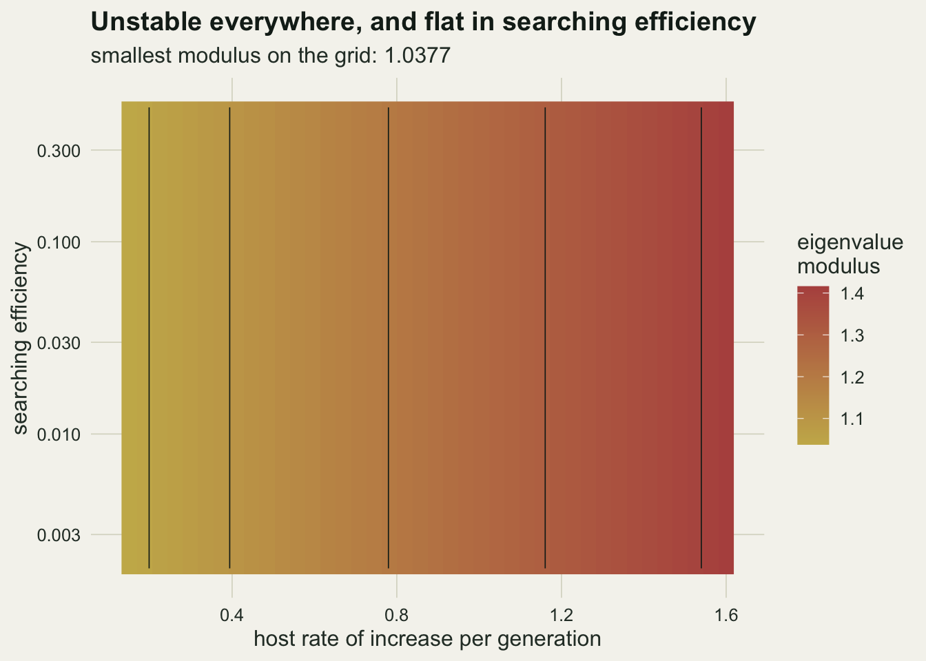
The cancellation is exact, and the algebra says so without the grid. The searching efficiency enters the Jacobian only through the product of itself with the equilibrium host density, and the equilibrium host density is itself inversely proportional to it, so the product is lam * log(lam) / (lam - 1) under random attack and carries no efficiency at all. That product is also the determinant of the Jacobian, and a determinant is the product of the two eigenvalues, so the larger modulus is at least the square root of the determinant.
det_closed <- function(lam, clump)
  if (is.infinite(clump)) lam * log(lam) / (lam - 1) else
    clump * lam * (1 - lam^(-1 / clump)) / (lam - 1)
probe <- expand.grid(lam = exp(seq(0.01, 3, length.out = 150)),
                     att = c(0.002, 0.05, 0.5), clump = c(0.5, 1, 2, Inf))
probe$num <- mapply(function(l, a, k) det(hp_jac(l, a, k)),
                    probe$lam, probe$att, probe$clump)
probe$ana <- mapply(det_closed, probe$lam, probe$clump); lam_probe_hi <- max(probe$lam)
nb_rows <- is.infinite(probe$clump); one_rows <- probe$clump == 1
det_err <- max(abs(probe$num - probe$ana) / probe$ana); n_probe <- nrow(probe)
nb_det_min <- min(probe$num[nb_rows]); one_dev <- max(abs(probe$num[one_rows] - 1))
Over 1800 combinations of host rate of increase, searching efficiency and clumping, reaching a host multiplier of 20.1 per generation, the numerical determinant matches that closed form to a worst relative error of 1.9e-14. Under random attack its smallest value on the probe is 1.0050, and the closed form exceeds one for every host multiplier above one, because lam * log(lam) exceeds lam - 1 there and equals it only in the limit of no growth. A determinant above one leaves no room for both eigenvalues inside the unit circle at any searching efficiency, so the instability belongs to the model and not to the parameters that happened to be tried.
Eigenvalues are an assertion about a linear approximation. The independent measurement is to run the map from a state displaced slightly from the equilibrium and watch the displacement grow. If the linearisation is right, the logarithm of the displacement should be linear in generation number with slope equal to the logarithm of the modulus, for as long as the displacement stays small.
run_map <- function(h0, p0, lam, att, clump, ngen) {
  out <- matrix(NA_real_, ngen + 1, 2)
  out[1, ] <- c(h0, p0)
  for (i in seq_len(ngen)) out[i + 1, ] <- hp_step(out[i, ], lam, att, clump)
  out
}

lam_ref <- exp(0.6); att_ref <- 0.05; eq_ref <- hp_eq(lam_ref, att_ref, Inf)
delta0 <- 1e-9; n_gen <- 110; burn_lin <- 10

path_nb <- run_map(eq_ref[["H"]] * (1 + delta0), eq_ref[["P"]],
                   lam_ref, att_ref, Inf, n_gen)
dev_rel <- sqrt(((path_nb[, 1] - eq_ref[["H"]]) / eq_ref[["H"]])^2 +
                ((path_nb[, 2] - eq_ref[["P"]]) / eq_ref[["P"]])^2)
gen_id <- 0:n_gen; keep <- gen_id >= burn_lin

fit_dev <- lm(log(dev_rel[keep]) ~ gen_id[keep])
slope_sim <- unname(coef(fit_dev)[2]); mod_sim <- exp(slope_sim)
mod_ana <- hp_modulus(lam_ref, att_ref, Inf)
mod_gap <- abs(mod_sim - mod_ana) / mod_ana
dev_end <- max(dev_rel); fit_r2 <- summary(fit_dev)$r.squared
Starting the host at a relative displacement of 1e-09 and running 110 generations, the displacement ends at 0.0083 of the equilibrium, so the whole path stays in the regime where a linear approximation is meaningful. The first 10 generations are dropped, because the initial displacement is along the host axis rather than along the leading eigenvector and the first few steps are the rotation onto it.
The fitted slope is 0.1425 per generation, which exponentiates to a per generation multiplier of 1.1531. The eigenvalue modulus is 1.1532. The two differ by 7.2e-05 in relative terms. Two measurements that share only the map and the equilibrium, both of which the check above validated separately, agree to four significant figures, and the residual wobble around the fitted line (the fit’s r squared is 0.9993) is the rotation of the complex eigenvalue pair, not a drift in the growth rate.
dev_dat <- data.frame(gen = gen_id, dev = dev_rel)
ggplot(dev_dat[keep, ], aes(gen, dev)) +
  geom_point(size = 1.3, colour = te_ink) +
  geom_line(aes(y = exp(predict(fit_dev))), colour = te_forest, linewidth = 0.9) +
  scale_y_log10() +
  labs(x = "generation", y = "relative displacement from equilibrium",
       title = "The displacement grows geometrically",
       subtitle = sprintf("fitted multiplier %.4f against eigenvalue modulus %.4f",
                          mod_sim, mod_ana)) +
  theme_datasheet()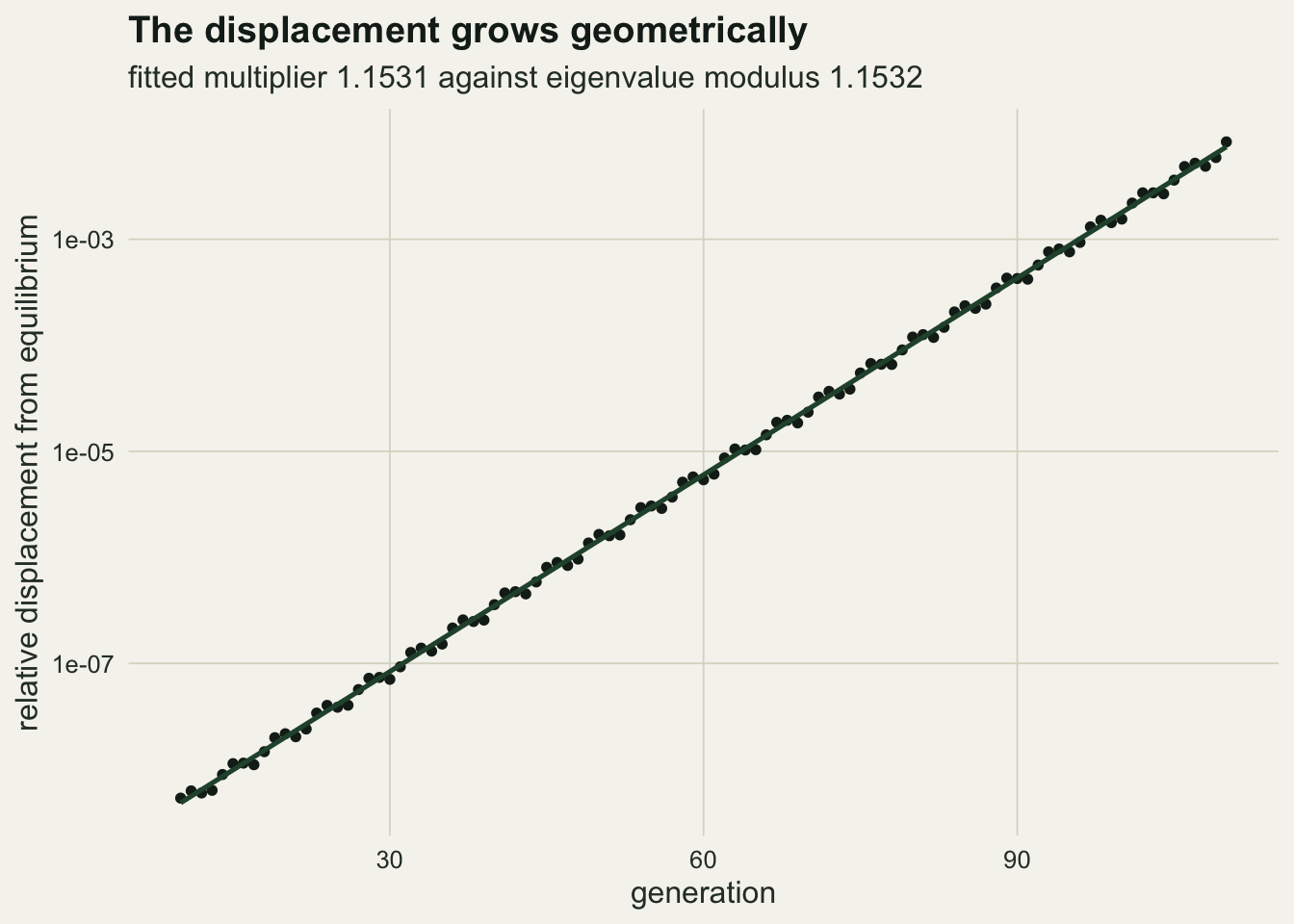
Aggregated attack crosses the threshold at a clumping of one
Random attack is the assumption doing the damage, not the parameter values. If wasps search patchily, or hosts differ in exposure, some hosts run a much higher risk than the average and others run almost none, and the fraction escaping is larger than the Poisson zero term for the same mean attack rate. May 1978 replaced the Poisson with a negative binomial, giving the escape function (1 + a * P / k)^(-k), where small k means strongly aggregated attack and k tending to infinity recovers random search. Hassell and May 1973 had already shown that non-random attack on a patchy host distribution was stabilising; the 1978 form is the phenomenological version that has one parameter and a closed form equilibrium.
k_star_of <- function(lam, att)
  uniroot(function(kk) hp_modulus(lam, att, kk) - 1, c(0.3, 3), tol = 1e-12)$root

k_set <- expand.grid(lam = exp(c(0.3, 0.6, 1.0, 1.5)), att = c(0.01, 0.05, 0.2))
k_star_all <- mapply(k_star_of, k_set$lam, k_set$att)

k_lin <- k_star_of(lam_ref, att_ref); k_lin_dev <- max(abs(k_star_all - 1))
n_k_combo <- length(k_star_all)
mod_at_half <- hp_modulus(lam_ref, att_ref, 0.5)
mod_at_two <- hp_modulus(lam_ref, att_ref, 2)
n_study <- 20; grow_two <- mod_at_two^n_study; grow_min <- mod_min^n_study
lam_panel <- exp(c(0.3, 0.6, 1.2))
Solving for the clumping value at which the modulus equals one gives 1.000000 at the reference parameters. Repeating the root finding over 12 combinations of host rate of increase and searching efficiency, the largest departure from one anywhere is 1.9e-13. The same determinant identity says why it cannot move. Under aggregated attack the determinant is clump * lam * (1 - lam^(-1 / clump)) / (lam - 1), again with the searching efficiency divided out, and at a clumping of one the factor lam * (1 - 1 / lam) is lam - 1, so the whole expression is one at every host rate of increase. On the probe set above, the determinant at a clumping of one departs from one by at most 3.3e-16, and the trace there is 1 + 1 / lam, which is below two, so the discriminant is negative and the eigenvalues are a complex conjugate pair whose modulus is the square root of the determinant. The threshold is not approximately one, it is one, and it does not move with either parameter. Below it the modulus falls quickly: at a clumping of half the modulus is 0.8800, against 1.0719 at a clumping of two.
The threshold in the currency a survey can measure
The escape function is not an arbitrary curve. It is what comes out when each host’s risk is multiplied by a gamma distributed factor of mean one, and the Poisson escape is then averaged over that factor. The gamma’s shape parameter is the clumping value, so its squared coefficient of variation is exactly the reciprocal of the clumping value, and the stability threshold at a clumping of one is the threshold at a squared coefficient of variation of one. That is the rule Pacala, Hassell and May 1990 named as the CV squared rule: heterogeneity in risk stabilises the interaction once the squared coefficient of variation of risk across hosts exceeds one. That criterion is an approximation derived for a class of patchy host-parasitoid models; in the negative binomial form used here it is exact, for the reason just given: the gamma mixture fixes that quantity at the reciprocal of the clumping parameter.
The reciprocal relation in the paragraph above is algebra, and the Monte Carlo here is not a second search for the threshold. What it checks is the two steps the algebra rests on: that a gamma factor whose shape is the clumping parameter has a squared coefficient of variation equal to the reciprocal of that parameter, and that averaging the Poisson escape over such a factor reproduces the negative binomial escape function. The replication was fixed before the numbers were seen. Forty batches of twenty thousand draws put the Monte Carlo standard error on the squared coefficient of variation at a few thousandths, which is fine enough to see a departure from one of the size that would matter.
n_batch <- 40; n_draw <- 20000

set.seed(41)
cv2_batch <- replicate(n_batch, {
  risk <- rgamma(n_draw, shape = k_lin, rate = k_lin)
  var(risk) / mean(risk)^2
})
cv2_mean <- mean(cv2_batch); cv2_mcse <- sd(cv2_batch) / sqrt(n_batch)
cv2_z <- abs(cv2_mean - 1) / cv2_mcse

k_demo <- 0.5; p_demo <- hp_eq(lam_ref, att_ref, k_demo)[["P"]]
set.seed(42)
risk_demo <- rgamma(n_draw * 10, shape = k_demo, rate = k_demo)
esc_mc    <- mean(exp(-att_ref * p_demo * risk_demo))
esc_mcse  <- sd(exp(-att_ref * p_demo * risk_demo)) / sqrt(n_draw * 10)
esc_exact <- escape_prob(p_demo, att_ref, k_demo)
esc_gap   <- abs(esc_mc - esc_exact)
cv2_demo  <- var(risk_demo) / mean(risk_demo)^2
At the threshold clumping the measured squared coefficient of variation of risk is 1.0005 with a Monte Carlo standard error of 0.0023, which is 0.2 standard errors from one. The mixture identity holds too: drawing risk factors at a clumping of 0.5 and averaging the Poisson escape over them gives 0.5488 with a standard error of 7.7e-04, against the closed form 0.5488, a gap of 2.5e-05. The same draws have a squared coefficient of variation of 1.998, above one, and that is the parameter region where the interaction persists.
Hassell and May 1974 made the ecological version of the same point with predators aggregating in patches of high host density. The phenomenological escape function does not say which mechanism generates the heterogeneity, only how much of it there has to be. The forty patch census in the opening is the design that estimates that amount: the model itself has no space in it, and the patches enter only as the spread in per host risk that the clumping parameter summarises.
The simulation puts the threshold below where the linearisation puts it
The threshold found above came from a linearisation. The independent way to find it is to simulate: fix a settling tolerance, run the map from a displaced start, discard a burn-in, and ask whether what is left is flat. The largest clumping value that still settles is the simulated threshold.
Three choices have to be stated. The starting displacement is five per cent of the equilibrium host density. The settling tolerance is a relative range of the host series below one part in a million over a window of two hundred generations. The burn-in is varied deliberately, because the point of the exercise is that it matters.
settle_win <- 200; settle_tol <- 1e-6; start_disp <- 0.05

has_settled <- function(clump, burn) {
  eq <- hp_eq(lam_ref, att_ref, clump)
  path <- run_map(eq[["H"]] * (1 + start_disp), eq[["P"]],
                  lam_ref, att_ref, clump, burn + settle_win)
  tail_h <- path[(burn + 1):(burn + settle_win + 1), 1]
  if (any(!is.finite(tail_h))) return(FALSE)
  diff(range(tail_h)) / eq[["H"]] < settle_tol
}

k_sim_of <- function(burn) {
  lo <- 0.5; hi <- 1.2
  for (i in 1:40) {
    mid <- (lo + hi) / 2
    if (has_settled(mid, burn)) lo <- mid else hi <- mid
  }
  (lo + hi) / 2
}

burn_short <- 500; burn_mid <- 2000; burn_long <- 8000
burn_set <- c(burn_short, burn_mid, burn_long)
k_sim_all <- vapply(burn_set, k_sim_of, 0)
k_sim_short <- k_sim_all[1]; k_sim_mid <- k_sim_all[2]; k_sim_long <- k_sim_all[3]
mod_sim_mid <- hp_modulus(lam_ref, att_ref, k_sim_mid)
k_gap_all <- k_lin - k_sim_all
k_gap_short <- k_gap_all[1]; k_gap_mid <- k_gap_all[2]; k_gap_long <- k_gap_all[3]
decay_need <- log(settle_tol / start_disp)
mod_bound_mid <- exp(decay_need / burn_mid)
With a burn-in of 500 generations the simulated threshold is 0.854, with 2000 generations it is 0.959, and with 8000 generations it is 0.989. The gap from the linearised threshold shrinks from 0.146 to 0.041 to 0.011.
The two measurements disagree, and the disagreement is a property of the simulation rather than of the model. Just below the threshold the modulus is just below one, so the displacement decays by an arbitrarily small factor per generation. Reaching the stated tolerance requires the logarithm of the decay to accumulate to -10.8 over the burn-in, so a burn-in of 2000 generations can certify only parameters whose modulus is below 0.9946. The modulus at the threshold the bisection actually returned is 0.9943, just inside that ceiling, which is what a burn-in-limited bisection should return. The linearised threshold is the exact one; the simulated threshold is a statement about how long anyone was willing to wait. Reporting the simulated value alone, without the burn-in, would look like a measurement and would be a description of the computing budget.
mod_dat <- do.call(rbind, lapply(lam_panel, function(l) {
  kk <- seq(0.3, 2.5, length.out = 300)
  data.frame(clump = kk,
             modulus = vapply(kk, function(z) hp_modulus(l, att_ref, z), 0),
             lam = sprintf("host rate %.1f per generation", log(l)))
}))

ggplot(mod_dat, aes(clump, modulus, colour = lam)) +
  annotate("rect", xmin = -Inf, xmax = 1, ymin = -Inf, ymax = 1,
           fill = te_forest, alpha = 0.10) +
  annotate("text", x = 0.58, y = 0.71, label = "stable side",
           colour = te_body, size = 3.6, hjust = 0) +
  geom_hline(yintercept = 1, linetype = "dashed", colour = te_body,
             linewidth = 0.5) +
  geom_line(linewidth = 0.9) +
  annotate("point", x = k_sim_mid, y = 1, shape = 4, size = 3.4,
           stroke = 1.2, colour = te_rust) +
  scale_colour_manual(values = c(te_gold, te_forest, te_rust), name = NULL) +
  labs(x = "clumping parameter of the attack distribution",
       y = "leading eigenvalue modulus",
       title = "The threshold sits at a clumping of one",
       subtitle = sprintf("red cross: simulated threshold %.3f after a burn-in of %d generations",
                          k_sim_mid, burn_mid)) +
  theme_datasheet() +
  theme(legend.position = "bottom")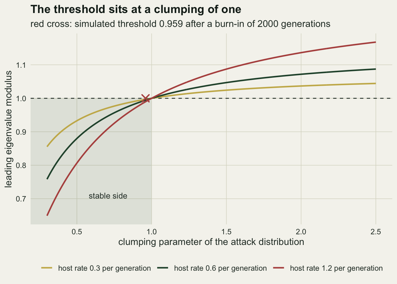
Stability is paid for in host density
A stable equilibrium is not the same thing as a suppressed pest. The equilibrium host density under aggregated attack, divided by the Nicholson-Bailey density at the same host rate and searching efficiency, is clump * (lam^(1 / clump) - 1) / log(lam), a quantity that is one when attack is random and grows without bound as attack becomes more aggregated.
host_ratio <- function(lam, clump) clump * (lam^(1 / clump) - 1) / log(lam)

k_high <- 0.9; k_mid <- 0.5; k_low <- 0.3
ratio_high <- host_ratio(lam_ref, k_high); ratio_mid <- host_ratio(lam_ref, k_mid)
ratio_low <- host_ratio(lam_ref, k_low); ratio_at_one <- host_ratio(lam_ref, 1)

rate_slow <- log(lam_panel[1]); rate_fast <- log(lam_panel[3])
ratio_slow <- host_ratio(lam_panel[1], k_low)
ratio_fast <- host_ratio(lam_panel[3], k_low)
k_seq_price <- seq(0.2, 1.6, length.out = 200)
price_dat <- do.call(rbind, lapply(lam_panel, function(l)
  data.frame(clump = k_seq_price, ratio = host_ratio(l, k_seq_price),
             lam = sprintf("host rate %.1f per generation", log(l)))))
At the reference host rate of increase, a clumping of 0.9 leaves the equilibrium host density 1.42 times the Nicholson-Bailey value, a clumping of 0.5 raises it to 1.93 times, and a clumping of 0.3 to 3.19 times. The cost rises with the host’s own rate of increase: at a clumping of 0.3 the multiplier is 1.72 for the slowest host in the panel (rate of increase 0.3) and 13.4 for the fastest (rate of increase 1.2). Exactly at the threshold the multiplier is already 1.37, so the interaction is never both stable and as suppressed as the unstable case would have been.
That is the trade a biological control programme is making without necessarily knowing it. Heterogeneity in attack is what keeps the wasp and the host in the same field from one decade to the next, and the same heterogeneity is what leaves a reservoir of hosts that the wasp never reaches. Hassell 2000 works through the field evidence for both halves.
ggplot(price_dat, aes(clump, ratio, colour = lam)) +
  geom_vline(xintercept = 1, linetype = "dashed", colour = te_body,
             linewidth = 0.5) +
  geom_line(linewidth = 0.9) +
  scale_colour_manual(values = c(te_gold, te_forest, te_rust), name = NULL) +
  scale_y_log10() +
  labs(x = "clumping parameter of the attack distribution",
       y = "equilibrium host density, multiple of Nicholson-Bailey",
       title = "What the stability costs",
       subtitle = "dashed line: the stability threshold") +
  theme_datasheet() +
  theme(legend.position = "bottom")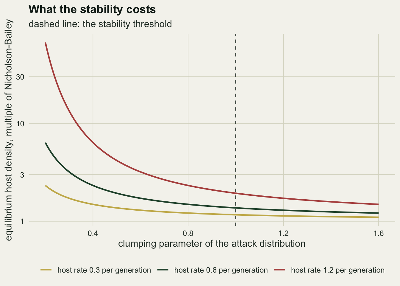
What to report
Give the stability criterion you used and the time convention it belongs to. A modulus below one and a negative real part are different tests, they apply to different models, and quoting one while having computed the other is a silent error that no software will catch.
Report the modulus, not a verdict. A modulus of 1.0719 and a modulus of 1.0377 are both unstable, but over the 20 generations of the census in the opening the first multiplies a displacement by 4.0 and the second by 2.1. The first would be visible as a departure; the second would look like noise.
If a threshold is claimed, locate it twice. The linearised value and the simulated value here differ by 0.041 at a burn-in of 2000 generations, and the difference is entirely explained by the burn-in. A threshold reported from simulation without its burn-in, its settling tolerance and its starting displacement cannot be reproduced or criticised.
State the heterogeneity as a squared coefficient of variation rather than as a clumping parameter when the audience is a field one. The clumping parameter is an artefact of choosing a negative binomial; the squared coefficient of variation of risk is measurable from a parasitism survey, and the threshold sits at one in both currencies.
Report the equilibrium host density alongside the stability verdict. Stability and suppression pull in opposite directions in this model, and a control programme that reports only that the system persists has reported half of the result.
Honest limits
The model has no host density dependence. Real hosts run out of food, and adding a host carrying capacity changes the picture substantially: the equilibrium becomes stable over a range of parameters even with random attack, and the threshold measured here is a threshold for the density independent case only. The choice is deliberate, because the point is what attack heterogeneity does on its own, but nothing here should be carried to a system where the host is near its own ceiling without redoing the algebra.
Local stability is all that has been measured. The modulus governs the fate of small displacements. It says nothing about what happens to a displacement of the size the leaf miner census actually shows, and a locally stable equilibrium can sit inside a small basin with wild dynamics outside it. Measuring that would need the basin boundary, not the Jacobian.
One wasp per parasitised host, one generation of delay and no overlap between generations are all assumptions. Gregarious parasitoids, partial voltinism and overwintering pools each add a state variable, and the two by two eigenvalue problem becomes larger, where the intuition that only the clumping parameter matters does not survive without checking.
The negative binomial escape function is phenomenological, and the CV squared rule stated over it is a generalisation rather than a consequence: Pacala, Hassell and May 1990 derived that criterion as an approximation holding across a family of patchy host-parasitoid models, several of which have no closed form escape function at all, so the exactness reported here is exactness within one member of that family. The escape function packages every source of heterogeneity into one number, whether that heterogeneity comes from the wasp aggregating in profitable patches, from hosts differing in concealment, or from the wasp’s own egg limitation. Those mechanisms differ in whether the heterogeneity tracks host density, and that distinction is the difference between the host density dependent and host density independent forms that the literature separates carefully. The stabilising effect measured here does not require the heterogeneity to track host density at all.
Finally, the simulated threshold is reported at one host rate of increase and one searching efficiency. The linearised threshold was checked over 12 parameter combinations and did not move, so there is reason to think the simulated shortfall behaves the same way everywhere, but that was not measured, and the burn-in needed for a given tolerance does depend on how fast the modulus falls away from one.
References
Nicholson AJ, Bailey VA 1935 Proceedings of the Zoological Society of London 105(3):551-598 (10.1111/j.1096-3642.1935.tb01680.x)
Hassell MP, May RM 1973 Journal of Animal Ecology 42(3):693 (10.2307/3133)
Hassell MP, May RM 1974 Journal of Animal Ecology 43(2):567 (10.2307/3384)
May RM 1978 Journal of Animal Ecology 47(3):833 (10.2307/3674)
Pacala SW, Hassell MP, May RM 1990 Nature 344(6262):150-153 (10.1038/344150a0)
Hassell MP 2000 The Spatial and Temporal Dynamics of Host-Parasitoid Interactions (ISBN 9780198540885)