---
title: "Food web structure: connectance and trophic level"
description: "Build a food web in R and measure its structure: connectance, trophic levels and food-chain length, and why the trophic level you report is a modelling choice."
date: "2026-06-21 14:00"
date-modified: "2026-10-07"
categories: [R, food webs, ecological networks, community ecology, ecology tutorial]
image: thumbnail.png
image-alt: "A directed food web drawn with species arranged by trophic level, from basal plants at the bottom to an eagle at the top."
---
*Corrected 7 October 2026: the caption of the trophic-level spread figure implied that omnivores in general span four levels, and its alt text gave the fox a wide gap; both now say that only the Raven has a wide spread and that no other species spans more than one level.*
A food web is a directed graph: a set of species and a record of who eats whom. Once you write it as a matrix, the whole toolbox of network structure opens up, and two numbers do most of the early work. Connectance says how densely the species are linked, and trophic level says how far up the chain each species sits. Both are easy to compute in a few lines of base R, and both hide a decision that changes the answer. This post builds a small web, measures its structure, and shows why the single most quoted food-web number, the trophic level, is not one number at all.
## A web as a matrix
Store the web as a square matrix `A` where `A[i, j] = 1` means species `i` eats species `j`. A row is a diet (what a species eats); a column is a predator list (what eats a species). We will use a small terrestrial web with two plants and a detritus pool, a set of herbivores, and predators up to three apex consumers with very different feeding habits.
```{r}
#| label: build-web
sp <- c("Grass","Sedge","Detritus","Vole","Hare","Grasshopper","Beetle",
        "Weasel","Shrew","Fox","Kestrel","Buzzard","Raven","Eagle")
S <- length(sp)

# prey list: what each species eats (by index)
prey <- list(
  integer(0),  # Grass      (basal)
  integer(0),  # Sedge      (basal)
  integer(0),  # Detritus   (basal)
  c(1, 2),     # Vole
  c(2, 3),     # Hare
  c(1, 3),     # Grasshopper
  c(1, 2),     # Beetle
  c(4, 6, 7),  # Weasel
  c(6, 7),     # Shrew
  c(4, 5, 8),  # Fox
  c(6, 7, 9),  # Kestrel
  c(8, 9, 10), # Buzzard
  c(3, 12),    # Raven   (detritus and buzzard: a broad scavenger)
  c(10)        # Eagle   (a fox specialist)
)

A <- matrix(0L, S, S, dimnames = list(sp, sp))
for (i in seq_len(S)) if (length(prey[[i]])) A[i, prey[[i]]] <- 1L

L <- sum(A)          # number of feeding links
C <- L / S^2         # directed connectance
c(species = S, links = L, connectance = round(C, 3))
```
The web has `r S` species and `r L` links. Connectance is the fraction of all possible links that are realised. There are several conventions; the most common is directed connectance, `C = L / S^2`, which here gives `r round(C, 3)`. Real food webs sit mostly between about 0.03 and 0.3, so this small web is unremarkable in density.
## Who sits where
Three roles fall out of the row and column sums. A basal species eats nothing in the web (row sum zero); a top species is eaten by nothing (column sum zero); everything else is intermediate. Two companion measures describe the link load: generality is the mean number of prey per consumer, and vulnerability is the mean number of predators per resource.
```{r}
#| label: roles
gen <- rowSums(A)              # generality: number of prey
vul <- colSums(A)              # vulnerability: number of predators
basal <- which(gen == 0)
top   <- which(vul == 0)
inter <- which(gen > 0 & vul > 0)

data.frame(
  role  = c("basal", "intermediate", "top"),
  count = c(length(basal), length(inter), length(top))
)
c(mean_generality   = round(mean(gen[gen > 0]), 2),
  mean_vulnerability = round(mean(vul[vul > 0]), 2),
  linkage_density    = round(L / S, 2))
```
The web has `r length(basal)` basal species, `r length(inter)` intermediate, and `r length(top)` top. On average a consumer eats `r round(mean(gen[gen>0]), 2)` species and a resource is eaten by `r round(mean(vul[vul>0]), 2)`. Linkage density (the ratio `L / S`, here `r round(L/S, 2)`) is the average number of links per species and is a common alternative to connectance when comparing webs of different sizes.
```{r}
#| label: fig-web
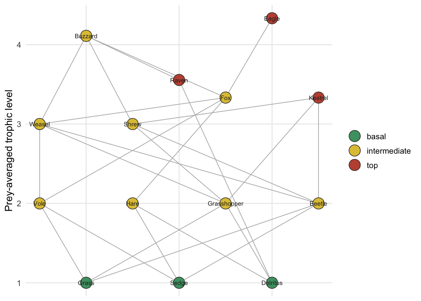
#| fig-cap: "The food web, with species placed at their prey-averaged trophic level and coloured by role. Grey lines are feeding links."
#| fig-alt: "Network diagram: three basal species at trophic level one, herbivores near two, and predators rising through a fox and a raven to a buzzard and an eagle at the top, connected by grey feeding links."
#| fig-width: 7
#| fig-height: 5
library(ggplot2)

# prey-averaged trophic level for vertical placement
Wmat <- A / pmax(rowSums(A), 1)
tl_pa <- solve(diag(S) - Wmat, rep(1, S))

role <- ifelse(gen == 0, "basal", ifelse(vul == 0, "top", "intermediate"))
set.seed(1)
# horizontal spread within trophic bands to reduce overlap
xpos <- ave(tl_pa, round(tl_pa), FUN = function(z) seq_along(z) - mean(seq_along(z)))
nodes <- data.frame(sp = sp, x = xpos, y = tl_pa, role = role)

edges <- do.call(rbind, lapply(seq_len(S), function(i) {
  if (!length(prey[[i]])) return(NULL)
  data.frame(x = nodes$x[prey[[i]]], y = nodes$y[prey[[i]]],
             xend = nodes$x[i], yend = nodes$y[i])
}))

ggplot() +
  geom_segment(data = edges, aes(x, y, xend = xend, yend = yend),
               colour = "grey72", linewidth = 0.4) +
  geom_point(data = nodes, aes(x, y, fill = role), shape = 21,
             size = 6, colour = "grey25") +
  geom_text(data = nodes, aes(x, y, label = sp), size = 2.6, colour = "grey15",
            nudge_y = 0.11, vjust = 0) +
  scale_fill_manual(values = c(basal = "#4c9f70", intermediate = "#e0c341",
                               top = "#c1523f")) +
  scale_y_continuous(expand = expansion(mult = c(0.06, 0.10))) +
  labs(x = NULL, y = "Prey-averaged trophic level", fill = NULL) +
  theme_minimal(base_size = 12) +
  theme(panel.grid.minor = element_blank(),
        axis.text.x = element_blank(),
        plot.background = element_rect(fill = "#f5f4ee", colour = NA),
        panel.background = element_rect(fill = "#f5f4ee", colour = NA))
```
## Three trophic levels, one web
Trophic level is meant to answer a simple question: how many steps of eating separate a species from the primary producers? The trouble is that there are at least three sensible ways to count those steps, and for anything that eats across levels they disagree.
The **prey-averaged** trophic level (the field standard since Williams and Martinez) sets basal species to 1 and every consumer to one plus the mean trophic level of its prey. It is the solution of a linear system, `(I - W) t = 1`, where `W` is the diet matrix with each consumer row scaled to sum to one.
The **shortest-path** level counts the shortest chain from a species down to a basal resource, so a fox that eats a rabbit and also nibbles carrion is only two steps from a plant.
The **longest-chain** level counts the longest such chain, so the same fox can sit near the top if one of its prey sits atop a long chain.
```{r}
#| label: trophic-levels
# (1) prey-averaged: t = 1 + W t, basal = 1  ->  (I - W) t = 1
tl_pa <- solve(diag(S) - Wmat, rep(1, S))

# (2) shortest path to a basal species
tl_sp <- rep(NA_real_, S); tl_sp[basal] <- 1
repeat {
  changed <- FALSE
  for (i in setdiff(seq_len(S), basal)) {
    p <- prey[[i]]
    if (all(!is.na(tl_sp[p]))) {
      v <- 1 + min(tl_sp[p])
      if (is.na(tl_sp[i]) || v < tl_sp[i]) { tl_sp[i] <- v; changed <- TRUE }
    }
  }
  if (!changed) break
}

# (3) longest chain (this web is acyclic, so it is finite)
tl_lc <- rep(NA_real_, S); tl_lc[basal] <- 1
repeat {
  changed <- FALSE
  for (i in setdiff(seq_len(S), basal)) {
    p <- prey[[i]]
    if (all(!is.na(tl_lc[p]))) {
      v <- 1 + max(tl_lc[p])
      if (is.na(tl_lc[i]) || v != tl_lc[i]) { tl_lc[i] <- v; changed <- TRUE }
    }
  }
  if (!changed) break
}

data.frame(species = sp, prey_avg = round(tl_pa, 2),
           shortest = tl_sp, longest = tl_lc)
```
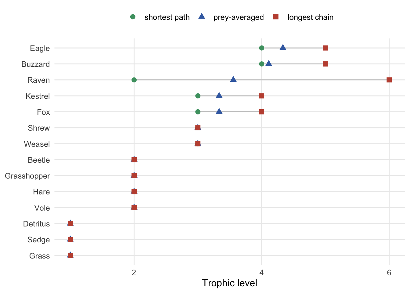
Look at the Raven. It eats detritus (a basal resource) and it eats the Buzzard (which sits atop a long chain). Its shortest-path level is `r tl_sp[13]`: it is one step from detritus, a primary consumer by that measure. Its longest-chain level is `r tl_lc[13]`: near the top. The prey-averaged level splits the difference at `r round(tl_pa[13], 2)`. That is not rounding noise; it is a four-level spread built into the web by a single omnivorous habit.
```{r}
#| label: fig-tl-spread
#| fig-cap: "Three trophic-level definitions for each species, ordered by the prey-averaged value. The line shows the spread: the omnivorous Raven spans four whole levels, and no other species spans more than one."
#| fig-alt: "Dot plot with species on the vertical axis and trophic level on the horizontal axis; each species has three points for the prey-averaged, shortest-path and longest-chain definitions, with a wide gap only for the raven and gaps of one level for the fox, kestrel, buzzard and eagle."
#| fig-width: 7
#| fig-height: 5
tl_long <- rbind(
  data.frame(sp = sp, tl = tl_pa, def = "prey-averaged"),
  data.frame(sp = sp, tl = tl_sp, def = "shortest path"),
  data.frame(sp = sp, tl = tl_lc, def = "longest chain")
)
ord <- sp[order(tl_pa)]
tl_long$sp <- factor(tl_long$sp, levels = ord)
tl_long$def <- factor(tl_long$def,
                       levels = c("shortest path", "prey-averaged", "longest chain"))

ggplot(tl_long, aes(tl, sp)) +
  geom_line(aes(group = sp), colour = "grey75", linewidth = 0.5) +
  geom_point(aes(colour = def, shape = def), size = 2.6) +
  scale_colour_manual(values = c("shortest path" = "#4c9f70",
                                 "prey-averaged" = "#3d6cb0",
                                 "longest chain" = "#c1523f")) +
  labs(x = "Trophic level", y = NULL, colour = NULL, shape = NULL) +
  theme_minimal(base_size = 12) +
  theme(panel.grid.minor = element_blank(),
        legend.position = "top",
        plot.background = element_rect(fill = "#f5f4ee", colour = NA),
        panel.background = element_rect(fill = "#f5f4ee", colour = NA))
```
The disagreement is not academic. Ask which species has the highest trophic level, a phrase that ends up in abstracts. The prey-averaged measure crowns the Eagle at `r round(max(tl_pa), 2)`, a clean specialist one link above the fox at `r round(tl_pa[10], 2)`. The longest-chain measure crowns the Raven at `r max(tl_lc)`, because one of the Raven's prey happens to sit atop the web's longest chain. Two defensible definitions, two different apex predators.
```{r}
#| label: rank-flip
c(prey_avg_highest = sp[which.max(tl_pa)],
  longest_highest  = sp[which.max(tl_lc)])
# rank agreement between definitions
round(c(pa_vs_shortest = cor(tl_pa, tl_sp, method = "spearman"),
        pa_vs_longest  = cor(tl_pa, tl_lc, method = "spearman"),
        shortest_vs_longest = cor(tl_sp, tl_lc, method = "spearman")), 3)
```
Across the whole web the three definitions correlate, but not perfectly: the prey-averaged and shortest-path rankings agree at `r round(cor(tl_pa, tl_sp, method="spearman"), 3)`, and the shortest-path and longest-chain at only `r round(cor(tl_sp, tl_lc, method="spearman"), 3)`. Omnivory is what pulls them apart, and omnivory is common in real webs.
## What to carry forward
Connectance and linkage density are unambiguous once you fix a counting convention, and they are the right first descriptors of a web. Trophic level is different. It reads like a measured quantity but it is a modelling choice, and for any omnivore the choice moves the answer by a level or more. Before you report a food-chain length or name a top predator, state which definition you used, and check that the claim survives the alternatives. The next post builds webs from scratch and asks a harder question: what simple rule reproduces the structure we just measured?
## Where to go next
The [niche model](../the-niche-model-of-food-webs/) shows that a single feeding axis generates realistic webs, while a random graph with the same connectance does not. For the undirected, two-mode case (plants and their pollinators rather than a directed food chain), see [bipartite network metrics](../bipartite-network-metrics/).
## References
Martinez ND 1992 American Naturalist 139(6):1208-1218 (10.1086/285382)
Williams RJ, Martinez ND 2004 American Naturalist 163(3):458-468 (10.1086/381964)
Pimm SL, Lawton JH, Cohen JE 1991 Nature 350:669-674 (10.1038/350669a0)
Dunne JA, Williams RJ, Martinez ND 2002 Proceedings of the National Academy of Sciences 99(20):12917-12922 (10.1073/pnas.192407699)
## Related tutorials
- [The niche model of food webs](../the-niche-model-of-food-webs/)
- [Stability and complexity in food webs](../stability-and-complexity-in-food-webs/)
- [Checking a food web analysis](../checking-a-food-web-analysis/)
- [Network robustness and secondary extinctions](../network-robustness-secondary-extinctions/)