---
title: "Checking a food web analysis"
description: "Three food web checks in R: sampling effort biases connectance, the null model sets how extreme a pattern looks, and stability hinges on self-regulation."
date: "2026-06-22 10:00"
date-modified: "2026-09-27"
categories: [R, food webs, model checking, community ecology, ecology tutorial]
image: thumbnail.png
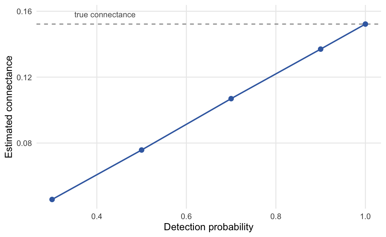
image-alt: "A single line chart for a food web analysis: estimated connectance climbs from about 0.05 at a detection probability of 0.3 to the dashed true value of about 0.15, which it reaches only at full detection."
---
*Corrected 27 September 2026: the self-regulation check said the web becomes stable only from d = 0.6 and put the predicted tipping point in a gap between rows; the table shows it is already stable at d = 0.4, and the switch sits near 0.37, close to the predicted value.*
The three previous posts built food webs, measured them, and asked whether they were stable. Each conclusion rested on something unstated. Connectance assumed the web was completely sampled. A structural claim assumed a particular null model. A stability verdict assumed a value for self-regulation that nobody measured. This post runs one check on each: the first two on a single web built with the niche model, the third on a random predator-prey community matrix, and each check turns a confident number into a conditional one.
```{r}
#| label: base-web
niche_web <- function(S, C) {
  n <- runif(S); beta <- 1 / (2 * C) - 1; r <- n * rbeta(S, 1, beta)
  r[which.min(n)] <- 0; centre <- runif(S, r / 2, n)
  A <- matrix(0L, S, S)
  for (i in seq_len(S)) A[i, n >= centre[i] - r[i] / 2 & n <= centre[i] + r[i] / 2] <- 1L
  A
}
role <- function(A) {
  g <- rowSums(A); v <- colSums(A)
  ifelse(g == 0, "basal", ifelse(v == 0, "top", "intermediate"))
}

set.seed(43)
S <- 30
A <- niche_web(S, 0.15)
true_role <- role(A)
c(species = S, links = sum(A), connectance = round(sum(A) / S^2, 3),
  basal = sum(true_role == "basal"), top = sum(true_role == "top"))
```
The web has `r sum(A)` links and a connectance of `r round(sum(A)/S^2, 3)`. Treat these as the truth, then see how each analysis would go wrong.
## Check 1: connectance depends on how hard you looked
A real web is assembled from observation, and no survey catches every feeding link. Suppose each true link is detected with probability `p`. Rebuild the web at several detection levels and recompute connectance and species roles.
```{r}
#| label: sampling
set.seed(101)
ps <- c(0.3, 0.5, 0.7, 0.9, 1.0)
sampled <- t(sapply(ps, function(p) {
  z <- t(replicate(400, {
    D <- A * (matrix(runif(S * S), S, S) < p)   # keep each true link w.p. p
    rr <- role(D)
    c(connectance = sum(D) / S^2,
      basal = sum(rr == "basal"),
      top   = sum(rr == "top"),
      misclassified = mean(rr != true_role))
  }))
  colMeans(z)
}))
data.frame(detection = ps, round(sampled, 3))
```
At full detection the connectance is the true `r round(sum(A)/S^2, 3)`. At 30% detection it reads `r round(sampled[1, "connectance"], 3)`, under a third of the truth, because most links are simply missed. The roles drift too: species that lose all their detected prey look basal, and the basal count climbs steadily as sampling worsens. At 30% detection, `r round(100 * sampled[1, "misclassified"])`% of species are placed in the wrong role. Connectance is not a property of a web alone; it is a property of a web and a sampling effort, and comparing it across studies that sampled differently compares the effort as much as the ecology.
```{r}
#| label: fig-sampling
#| fig-cap: "Estimated connectance against detection probability, for a web whose true connectance is fixed."
#| fig-alt: "Rising curve of estimated connectance against detection probability, well below the true value at low detection and reaching it only at full detection, marked by a dashed horizontal line."
#| fig-width: 6.5
#| fig-height: 4
library(ggplot2)
sdf <- data.frame(detection = ps, connectance = sampled[, "connectance"])
Ctrue <- sum(A) / S^2

ggplot(sdf, aes(detection, connectance)) +
  geom_hline(yintercept = Ctrue, linetype = "dashed", colour = "grey55") +
  geom_line(colour = "#3d6cb0", linewidth = 0.8) +
  geom_point(colour = "#3d6cb0", size = 2.4) +
  annotate("text", x = 0.35, y = Ctrue + 0.006, label = "true connectance",
           hjust = 0, size = 3.4, colour = "grey35") +
  labs(x = "Detection probability", y = "Estimated connectance") +
  theme_minimal(base_size = 12) +
  theme(panel.grid.minor = element_blank(),
        plot.background = element_rect(fill = "#f5f4ee", colour = NA),
        panel.background = element_rect(fill = "#f5f4ee", colour = NA))
```
## Check 2: significance is only as good as the null
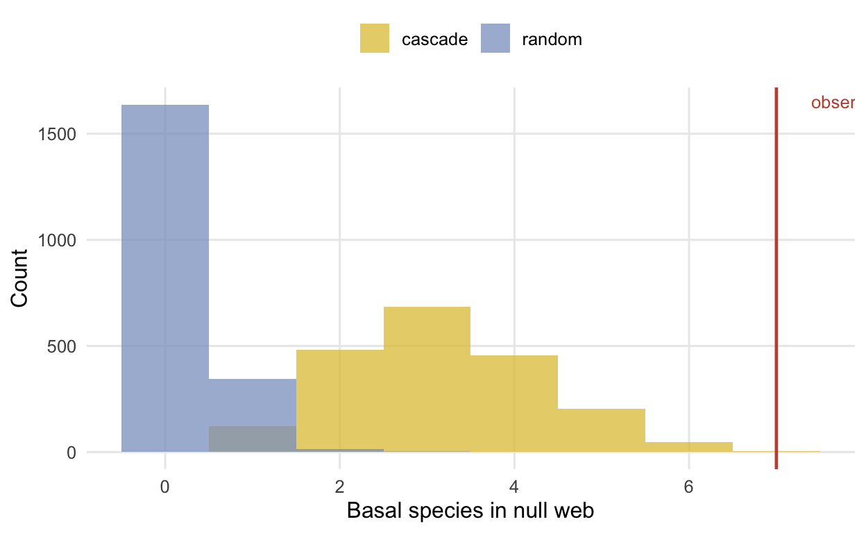
Say the web has `r sum(true_role == "basal")` basal species and you want to know whether that is more than expected by chance. The answer depends entirely on what "chance" means. Compare the observed count against two nulls that both keep the number of species and match the observed number of links: a random graph that scatters exactly that many links anywhere, and a cascade model that respects a feeding order and hits the link count only on average.
```{r}
#| label: nulls
random_L  <- function(S, L) { M <- matrix(0L, S, S); M[sample(S * S, L)] <- 1L; M }
cascade_L <- function(S, L) {
  p <- L / (S * (S - 1) / 2); M <- matrix(0L, S, S)
  for (i in 2:S) for (j in 1:(i - 1)) if (runif(1) < p) M[i, j] <- 1L
  M
}
obs_basal <- sum(true_role == "basal"); L <- sum(A)

set.seed(202)
rand_basal <- replicate(2000, sum(rowSums(random_L(S, L)) == 0))
casc_basal <- replicate(2000, sum(rowSums(cascade_L(S, L)) == 0))

data.frame(
  null = c("random", "cascade"),
  mean_basal = round(c(mean(rand_basal), mean(casc_basal)), 2),
  sd_basal   = round(c(sd(rand_basal),   sd(casc_basal)),   2),
  z_observed = round(c((obs_basal - mean(rand_basal)) / sd(rand_basal),
                       (obs_basal - mean(casc_basal)) / sd(casc_basal)), 1),
  p_one_sided = round(c(mean(rand_basal >= obs_basal),
                        mean(casc_basal >= obs_basal)), 3)
)
```
Against the random null the observed `r obs_basal` basal species is wildly significant: the random graph almost never leaves a species without prey, so its expected basal count is near zero and the observed value sits `r round((obs_basal - mean(rand_basal))/sd(rand_basal), 1)` standard deviations above it. Against the cascade null, which builds an ordered web and therefore produces basal species naturally, the same observation is `r round((obs_basal - mean(casc_basal))/sd(casc_basal), 1)` standard deviations out, a one-sided p of `r round(mean(casc_basal >= obs_basal), 3)`. Same data, same statistic, two nulls, and how far out the count sits changes once the null stops being absurd. The random null is the wrong one here, because having some producers is not the pattern you are testing; it is a basic feature any web must have. A significance star means nothing until the null is one that could plausibly have generated the data.
```{r}
#| label: fig-nulls
#| fig-cap: "Distribution of basal-species counts under two null models, with the observed count marked. The observed count sits far above everything the random null produced here, and in the upper tail of the cascade null."
#| fig-alt: "Two histograms of basal-species counts: the random null clustered near zero far from the observed line, the cascade null centred near three with the observed count of seven out in its upper tail."
#| fig-width: 6.5
#| fig-height: 4
nd <- rbind(data.frame(basal = rand_basal, null = "random"),
            data.frame(basal = casc_basal, null = "cascade"))

ggplot(nd, aes(basal, fill = null)) +
  geom_histogram(binwidth = 1, alpha = 0.75, position = "identity") +
  geom_vline(xintercept = obs_basal, colour = "#c1523f", linewidth = 0.8) +
  annotate("text", x = obs_basal - 0.3, y = Inf, vjust = 1.6, hjust = 1,
           label = "observed", size = 3.4, colour = "#c1523f") +
  scale_fill_manual(values = c("random" = "#8aa0c8", "cascade" = "#e0c341")) +
  labs(x = "Basal species in null web", y = "Count", fill = NULL) +
  theme_minimal(base_size = 12) +
  theme(panel.grid.minor = element_blank(),
        legend.position = "top",
        plot.background = element_rect(fill = "#f5f4ee", colour = NA),
        panel.background = element_rect(fill = "#f5f4ee", colour = NA))
```
## Check 3: the stability verdict rides on self-regulation
The stability calculation of the previous post compared interaction strength against the diagonal self-regulation `d`. That term sets the whole scale, and it is the parameter least likely to be measured. Fix a web and its interaction strengths, then vary only `d` and watch the verdict.
```{r}
#| label: self-regulation
stable <- function(M) max(Re(eigen(M, only.values = TRUE)$values)) < 0

set.seed(7)
Sp <- 50; Cp <- 0.20; sigma <- 0.35
E <- matrix(0, Sp, Sp)                       # one fixed predator-prey interaction structure
for (i in 1:(Sp - 1)) for (j in (i + 1):Sp) if (runif(1) < Cp) {
  E[i, j] <- abs(rnorm(1)); E[j, i] <- -abs(rnorm(1))
}

ds <- c(0.2, 0.3, 0.4, 0.6, 1.0)
verdict <- sapply(ds, function(dd) {
  M <- -dd * diag(Sp) + sigma * E
  c(self_regulation = dd,
    rightmost_eig = round(max(Re(eigen(M, only.values = TRUE)$values)), 3),
    stable = stable(M))
})
t(verdict)
```
Nothing about the web changed across those rows: the same species, the same interaction strengths, the same connectance. Only the assumed self-regulation moved. At weak self-regulation (`d` = 0.2 and 0.3) the system is unstable; at `d` = 0.4 and above it is stable. Because `d` shifts every eigenvalue by the same amount, the rightmost eigenvalue crosses zero near `d` = `r sprintf("%.2f", verdict["rightmost_eig", 1] + ds[1])`. The predicted tipping point, `sigma * sqrt(S * C) * (1 + rho)` with `rho = -2/pi` for paired predator-prey entries, is about `r round(sigma * sqrt(Sp * Cp) * (1 - 2/pi), 2)`, close to it. A paper that assumed strong self-regulation would report a stable web; one that assumed weak self-regulation would report an unstable one; and both would be describing the same interactions. Whenever a stability result appears, the first question is what diagonal was assumed, because that assumption, not the measured structure, often carries the conclusion.
## The common thread
Each check took a number that looked like a measured property of the web and showed it was really a property of the web plus a choice: how completely it was sampled, which null it was compared against, what self-regulation was assumed. None of these are failures of the methods; they are the conditions under which the methods mean what they say. Report the sampling effort with the connectance, the null with the significance, and the diagonal with the stability verdict, and the food web analysis becomes something a reader can actually check.
## Where to go next
This closes the food web series that began with [connectance and trophic level](../food-web-structure-connectance/), drew on the [niche model](../the-niche-model-of-food-webs/), and tested [stability and complexity](../stability-and-complexity-in-food-webs/). For the checking counterpart in undirected interaction networks, see [checking a network analysis](../checking-a-network-analysis/).
## References
Martinez ND, Hawkins BA, Dawah HA, Feifarek BP 1999 Ecology 80(3):1044-1055 (10.1890/0012-9658(1999)080[1044:EOSEOC]2.0.CO;2)
Dunne JA, Williams RJ, Martinez ND 2002 Proceedings of the National Academy of Sciences 99(20):12917-12922 (10.1073/pnas.192407699)
Williams RJ, Martinez ND 2004 American Naturalist 163(3):458-468 (10.1086/381964)
Allesina S, Tang S 2012 Nature 483(7388):205-208 (10.1038/nature10832)
## Related tutorials
- [Food web structure: connectance and trophic level](../food-web-structure-connectance/)
- [Network robustness and secondary extinctions](../network-robustness-secondary-extinctions/)
- [Stability and complexity in food webs](../stability-and-complexity-in-food-webs/)
- [Checking a network analysis](../checking-a-network-analysis/)