library(ggplot2)

te_paper  <- "#f5f4ee"
te_ink    <- "#16241d"
te_body   <- "#2c3a31"
te_forest <- "#275139"
te_rust   <- "#b5534e"
te_gold   <- "#c9b458"
te_line   <- "#dad9ca"

theme_datasheet <- function() {
  theme_minimal(base_size = 12) +
    theme(plot.background  = element_rect(fill = te_paper, colour = NA),
          panel.background = element_rect(fill = te_paper, colour = NA),
          panel.grid.major = element_line(colour = te_line, linewidth = 0.3),
          panel.grid.minor = element_blank(),
          text             = element_text(colour = te_body),
          plot.title       = element_text(colour = te_ink, face = "bold"),
          axis.text        = element_text(colour = te_body))
}Network robustness and secondary extinctions
R
ecological networks
extinction
statistics
ecology tutorial
Attack tolerance curves and R50 for pollination webs in base R, showing that R50 is a joint property of the web, the removal order and the dependence rule.
A pollination web gets published with an attack tolerance curve behind it. Plants are deleted one at a time, any pollinator left without a single remaining partner is counted as gone, and the curve of surviving pollinators against plants removed is boiled down to R50: the fraction of plants that has to disappear before half the pollinators have. The number then travels as a property of the community. This web is fragile, that one holds up.
Two decisions taken before a single plant was deleted are inside that number as well. The first is the order the plants go in. The second is the rule that decides when a pollinator with some partners left still counts as extinct. R50 is a joint property of all three, and the useful question is not which of them wins but how large each one is. This post measures all three with the same code, on one web and then on a set of fifteen.
A web to break
The web is built rather than borrowed, so its structure is known. Each pollinator gets a generality score and each plant an attractiveness score on the same axis; a link is likely when the two scores add up to enough. Multiplying by abundances and taking Poisson counts gives a weighted matrix with the one feature that matters here: degrees that vary a lot between species, which also makes the matrix look nested, since the specialists end up on the plants the generalists already use.
make_web <- function(n_poll, n_plant, alpha, theta, seed, total = 1200) {
  set.seed(seed)
  gener <- runif(n_poll)
  attra <- runif(n_plant)
  ab_p  <- exp(rnorm(n_poll, 0, 0.8))
  ab_l  <- exp(rnorm(n_plant, 0, 0.6))
  pr    <- plogis(alpha * (outer(gener, attra, "+") - theta))
  lam   <- outer(ab_p, ab_l) * pr
  lam   <- lam / sum(lam) * total
  wm    <- matrix(rpois(n_poll * n_plant, lam), n_poll, n_plant)
  wm    <- wm[rowSums(wm) > 0, , drop = FALSE]
  wm    <- wm[, colSums(wm) > 0, drop = FALSE]
  dimnames(wm) <- list(paste0("poll", seq_len(nrow(wm))),
                       paste0("plant", seq_len(ncol(wm))))
  wm
}

web_a <- make_web(45, 28, alpha = 10, theta = 1.5, seed = 20260813)
n_a <- nrow(web_a); p_a <- ncol(web_a)
deg_plant <- colSums(web_a > 0)
round(c(pollinators = n_a, plants = p_a,
        connectance = sum(web_a > 0) / (n_a * p_a),
        plant_degree_min = min(deg_plant), plant_degree_max = max(deg_plant)), 3)
pollinators plants connectance plant_degree_min
36.000 27.000 0.301 1.000
plant_degree_max
34.000 36 pollinators, 27 plants, connectance 0.30. Plant degree runs from 1 to 34, which is the heterogeneity the whole exercise depends on: deleting a plant that 34 pollinators use is a different event from deleting one at the bottom of that range. Degree, connectance and the weighted descriptors are all built by hand in bipartite network metrics from scratch; the same vocabulary is used here without reintroducing it.
The cascade itself is short. Delete a plant, recount each pollinator’s remaining links, retire the ones at zero, record the surviving fraction, repeat. Extinction is permanent, which comes for free because remaining degree only ever falls. The guard on the first line matters if you bring your own matrix: a pollinator with zero total strength makes the lost fraction undefined, which under the stochastic rule returns a curve of NA and under the all-or-nothing rule silently deflates it.
survivors <- function(wm, ord, b = Inf, u = NULL) {
  stopifnot(all(rowSums(wm) > 0))
  strength <- rowSums(wm)
  keep  <- rep(TRUE, ncol(wm))
  alive <- rep(TRUE, nrow(wm))
  out   <- numeric(length(ord) + 1)
  out[1] <- 1
  for (k in seq_along(ord)) {
    keep[ord[k]] <- FALSE
    remain <- rowSums(wm[, keep, drop = FALSE])
    lost   <- 1 - remain / strength
    alive  <- alive & (if (is.infinite(b)) remain > 0 else lost^b <= u)
    out[k + 1] <- mean(alive)
  }
  out
}

# R (Burgos et al 2007) is the area under the curve;
# R50 the removed fraction at half survival
r_index <- function(y) {
  x <- seq(0, 1, length.out = length(y))
  sum(diff(x) * (head(y, -1) + tail(y, -1)) / 2)
}
r50 <- function(y) {
  x <- seq(0, 1, length.out = length(y))
  i <- which(y <= 0.5)[1]
  if (i == 1) return(0)
  x[i - 1] + (y[i - 1] - 0.5) / (y[i - 1] - y[i]) * (x[i] - x[i - 1])
}

curve_most  <- survivors(web_a, order(deg_plant, decreasing = TRUE))
curve_least <- survivors(web_a, order(deg_plant))
round(c(R_most_connected_first = r_index(curve_most),
        R50_most_connected_first = r50(curve_most)), 3)
R_most_connected_first R50_most_connected_first
0.435 0.457 Take the most connected plants out first and the web loses half its pollinators by the time 46 per cent of the plants are gone, with area under the curve 0.44. That is the number an author would report if the question were framed as worst case. Frame it any other way and it changes.
The removal order sets the answer
Three orders on this one web, which are the three the literature actually uses (Memmott et al 2004; Dunne et al 2002): most connected first, least connected first, and random. Random removal is not one curve, so a set of orders is drawn once and reused for everything that follows.
set.seed(505)
n_rep    <- 2000
ord_mat  <- replicate(n_rep, sample(p_a))
rand_curves <- sapply(seq_len(n_rep), function(i) survivors(web_a, ord_mat[, i]))
rand_r50 <- apply(rand_curves, 2, r50)
xs <- seq(0, 1, length.out = p_a + 1)

order_tab <- data.frame(
  order = c("most connected first", "random (mean)", "least connected first"),
  R     = c(r_index(curve_most), mean(apply(rand_curves, 2, r_index)),
            r_index(curve_least)),
  R50   = c(r50(curve_most), mean(rand_r50), r50(curve_least)))
order_span <- mean(rand_r50) - r50(curve_most)
round(order_tab[, -1], 3)
R R50
1 0.435 0.457
2 0.828 0.892
3 0.976 0.980round(c(most_to_random_span = order_span,
mc_standard_error = sd(rand_r50) / sqrt(n_rep),
random_q10 = quantile(rand_r50, 0.1),
random_q90 = quantile(rand_r50, 0.9),
ceiling = (p_a - 0.5) / p_a), 3)most_to_random_span mc_standard_error random_q10.10% random_q90.90%
0.436 0.002 0.801 0.972
ceiling
0.981 band <- data.frame(x = xs,
lo = apply(rand_curves, 1, quantile, 0.1),
hi = apply(rand_curves, 1, quantile, 0.9),
mid = rowMeans(rand_curves))
lines_df <- data.frame(
x = rep(xs, 3), y = c(curve_most, band$mid, curve_least),
order = factor(rep(c("most connected first", "random (mean)",
"least connected first"), each = p_a + 1),
levels = c("most connected first", "random (mean)",
"least connected first")))
ggplot(lines_df, aes(x, y)) +
geom_ribbon(data = band, aes(x = x, ymin = lo, ymax = hi),
inherit.aes = FALSE, fill = te_gold, alpha = 0.3) +
geom_hline(yintercept = 0.5, linetype = "dashed", colour = te_body) +
geom_line(aes(colour = order), linewidth = 1) +
scale_colour_manual(values = c(te_rust, te_ink, te_forest)) +
labs(x = "fraction of plants removed", y = "fraction of pollinators surviving",
colour = NULL, title = "One web, three answers") +
theme_datasheet() +
theme(legend.position = "bottom")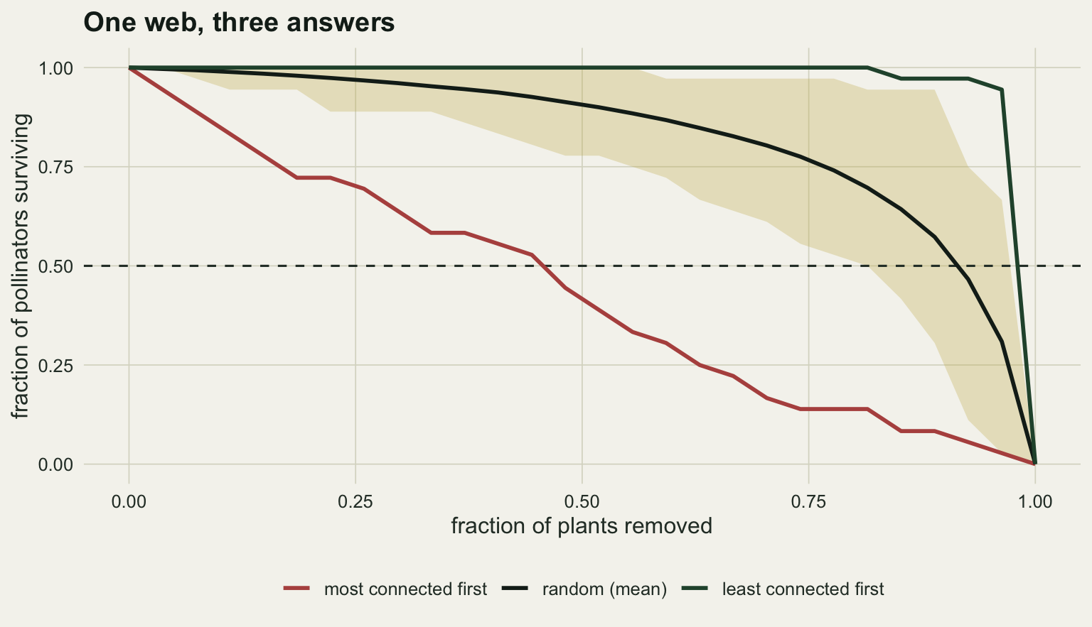
R50 reads 0.46, 0.89 and 0.98 on one fixed matrix. Nothing about the community changed between those three numbers; only the deletion sequence did.
The top of that range is a ceiling rather than a measurement. With 27 plants the largest R50 an interpolated curve can return is (p - 0.5) / p, here 0.981, and least connected first lands 0.001 below it. Its curve never really crosses one half either: it sits at 0.944 with one plant left and goes to zero on the final removal, so the reported crossing is an interpolation inside a single discontinuous drop. The span worth quoting is the one between most connected first and the random mean, where both endpoints are things the web actually did: 0.436 here.
The band is worth a look on its own. Across 2000 random orders R50 has a ten to ninety per cent range of 0.80 to 0.97, so even random removal, the one order that is not stacked in either direction, carries real spread. A paper that ran one random sequence has reported a draw from that distribution. The mean over 2000 replicates has a Monte Carlo standard error of 0.0015, so web A’s spans carry two safe decimals. The bank below runs a tenth of that replication per web, so its spans are good to about a hundredth and no further.
Between orders, between webs
The comparison that gives the point its teeth is against variation between webs, because comparing webs is what R50 is normally used for. Two more webs from the same generator go first, then a wider bank: three Erdos-Renyi webs with near-uniform degrees, three perfectly nested ones, three modular ones and three more from the generator. All of them are built from base R and the same cascade runs on all of them.
trim <- function(wm) {
  wm <- wm[rowSums(wm) > 0, , drop = FALSE]
  wm[, colSums(wm) > 0, drop = FALSE]
}
web_er <- function(n_poll, n_plant, fill, seed) {
  set.seed(seed)
  wm <- matrix(0, n_poll, n_plant)
  cells <- sample(n_poll * n_plant, round(fill * n_poll * n_plant))
  wm[cells] <- 1 + rpois(length(cells), 4)
  trim(wm)
}
web_nested <- function(n_poll, n_plant, seed) {
  set.seed(seed)
  k <- 1 + round((n_plant - 1) * sort(rbeta(n_poll, 0.7, 1.3)))
  trim(t(sapply(k, function(d) c(1 + rpois(d, 5), rep(0, n_plant - d)))))
}
web_modular <- function(n_poll, n_plant, n_mod, seed) {
  set.seed(seed)
  gp  <- sample(rep(seq_len(n_mod), length.out = n_poll))
  gl  <- sample(rep(seq_len(n_mod), length.out = n_plant))
  lam <- outer(gp, gl, function(a, b) ifelse(a == b, 3.2, 0.12))
  trim(matrix(rpois(n_poll * n_plant, lam), n_poll, n_plant))
}

bank <- list("generator A" = web_a,
             "generator B" = make_web(45, 28, alpha = 4,  theta = 1.0, seed = 4114),
             "generator C" = make_web(40, 24, alpha = 14, theta = 1.7, seed = 911))
for (s in 1:3) {
  bank[[paste("generator", s)]]   <- make_web(45, 28, alpha = 6 + 3 * s,
                                              theta = 1.1 + 0.2 * s, seed = 700 + s)
  bank[[paste("Erdos-Renyi", s)]] <- web_er(40, 26, fill = 0.14 + 0.06 * s, seed = 300 + s)
  bank[[paste("nested", s)]]      <- web_nested(40, 26, seed = 500 + s)
  bank[[paste("modular", s)]]     <- web_modular(40, 26, n_mod = 1 + s, seed = 900 + s)
}

bank_tab <- do.call(rbind, lapply(names(bank), function(nm) {
  wm <- bank[[nm]]
  dg <- colSums(wm > 0)
  set.seed(505)
  rc <- replicate(200, survivors(wm, sample(ncol(wm))))
  data.frame(web = nm, family = sub(" .*$", "", nm), plants = ncol(wm),
             connectance = sum(wm > 0) / (nrow(wm) * ncol(wm)),
             degree_cv = sd(dg) / mean(dg),
             R50_most = r50(survivors(wm, order(dg, decreasing = TRUE))),
             R50_random = mean(apply(rc, 2, r50)))
}))
bank_tab$order_span <- bank_tab$R50_random - bank_tab$R50_most

fam_tab <- do.call(rbind, lapply(split(bank_tab, bank_tab$family), function(d)
  data.frame(webs = nrow(d), connectance = mean(d$connectance),
             degree_cv = mean(d$degree_cv), R50_most = mean(d$R50_most),
             order_span = mean(d$order_span))))
web_span_most   <- diff(range(bank_tab$R50_most))
web_span_random <- diff(range(bank_tab$R50_random))
print(round(fam_tab, 3))
webs connectance degree_cv R50_most order_span
Erdos-Renyi 3 0.260 0.267 0.851 0.053
generator 6 0.371 0.730 0.534 0.380
modular 3 0.419 0.097 0.912 0.031
nested 3 0.391 0.785 0.313 0.584round(c(between_web_span_most = web_span_most,
between_web_span_random = web_span_random,
median_order_span = median(bank_tab$order_span),
webs_where_order_span_is_larger = sum(bank_tab$order_span > web_span_most)), 3) between_web_span_most between_web_span_random
0.759 0.106
median_order_span webs_where_order_span_is_larger
0.355 0.000 Start with the three webs from the one generator, which is about as much variation as a single study usually has. Their order spans are 0.44, 0.12 and 0.45, against a between-web span of 0.37 under most connected first. On two of the three the order moves R50 further than swapping the web does; on the third, the one with the most even plant degrees, it moves it far less. How much the analyst’s choice matters is itself a property of the web, which is the first thing a single headline number hides.
span_df <- bank_tab
span_df$web <- factor(span_df$web, levels = span_df$web[order(span_df$R50_most)])
pt_df <- data.frame(
  web   = rep(span_df$web, 2),
  value = c(span_df$R50_most, span_df$R50_random),
  ord   = factor(rep(c("most connected first", "random (mean)"),
                     each = nrow(span_df)),
                 levels = c("most connected first", "random (mean)")))

p_span <- ggplot(span_df) +
  geom_segment(aes(x = R50_most, xend = R50_random, y = web, yend = web),
               colour = te_gold, linewidth = 2.2) +
  geom_point(data = pt_df, aes(value, web, colour = ord), size = 2.6) +
  scale_colour_manual(values = c(te_rust, te_ink)) +
  labs(x = "R50", y = NULL, colour = NULL,
       title = "The web moves it further than the order does") +
  theme_datasheet() +
  theme(legend.position = "bottom")
p_span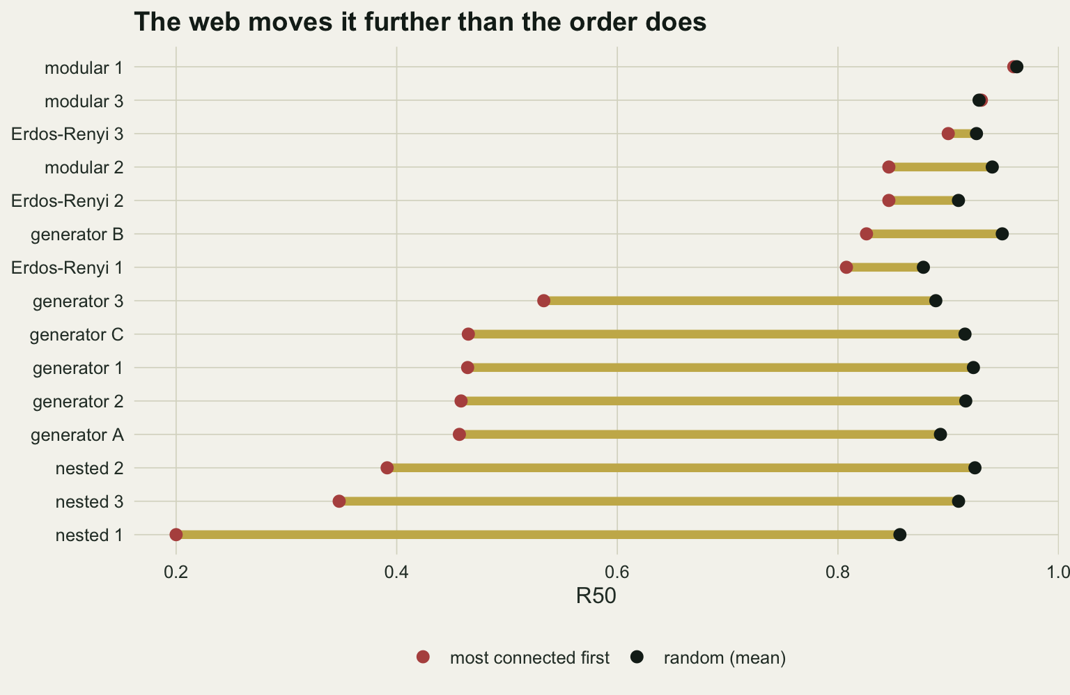
Across all 15 webs the picture turns over. R50 under most connected first spans 0.76, from 0.20 on a nested web to 0.96 on a modular one, while the median within-web order span is 0.36 and the largest is 0.66. The number of webs whose order span beats that between-web span is 0 out of 15. Given webs this varied the web wins, and a comparison resting on three siblings from one generator has it the wrong way round.
Two things keep the analyst’s choice in the argument. The order span is not noise: it correlates 0.93 with the coefficient of variation of plant degree, so it is small on the flat modular webs and at least 0.53 on each of the nested ones. The order choice is worth little on a web with even plant degrees and worth a great deal on one where a handful of plants carry a large share of the links. And hold the order fixed at random, the version most often reported, and the between-web span across the same fifteen webs falls to 0.11, about 2.9 plant-removal steps on a web the size of web A. On two of the three modular webs the order span comes out at or just below zero: with near-uniform plant degrees there is nothing for a degree-based order to exploit, and what is left is Monte Carlo noise in the random mean.
The dependence rule moves it almost as far again
The all-or-nothing rule is the most forgiving assumption available. A pollinator that has lost nine tenths of its visits and every partner but one is scored as fully alive. Nothing in pollination biology says that a bee which has lost its main forage plant is unaffected as long as one late-flowering shrub remains.
The softer rule below keeps the same cascade and changes only the survival test, in the spirit of Vieira and Almeida-Neto (2015) though simpler than their model. Let lost be the fraction of a pollinator’s original interaction strength that has gone with the deleted plants. Give each pollinator a tolerance threshold drawn once from a uniform, and retire it as soon as lost^b exceeds that threshold. The exponent b sets how forgiving the rule is: b of 1 means a pollinator that has lost half its strength has a one in two chance of being gone, and as b grows the rule slides back towards all-or-nothing, which is the limit at infinity. The three rules are run on the same 2000 removal orders as the section above and the same thresholds, so the comparison is paired and the differences are not a race between separate random draws.
set.seed(77)
u_mat <- replicate(n_rep, runif(n_a))
rule_r50 <- sapply(c(Inf, 3, 1), function(b)
  apply(sapply(seq_len(n_rep), function(i)
    survivors(web_a, ord_mat[, i], b = b, u = u_mat[, i])), 2, r50))
rule_lab <- c("all or nothing", "b = 3", "b = 1")
colnames(rule_r50) <- rule_lab
paired_drop <- rule_r50[, 1] - rule_r50[, 3]
round(colMeans(rule_r50), 3)
all or nothing b = 3 b = 1
0.892 0.708 0.495 round(c(paired_drop = mean(paired_drop),
mc_standard_error = sd(paired_drop) / sqrt(n_rep),
share_of_order_span = mean(paired_drop) / order_span), 3) paired_drop mc_standard_error share_of_order_span
0.398 0.004 0.913 mean_curves <- sapply(c(Inf, 3, 1), function(b)
rowMeans(sapply(seq_len(n_rep), function(i)
survivors(web_a, ord_mat[, i], b = b, u = u_mat[, i]))))
rule_df <- data.frame(x = rep(xs, 3), y = as.vector(mean_curves),
rule = factor(rep(rule_lab, each = p_a + 1),
levels = rule_lab))
ggplot(rule_df, aes(x, y, colour = rule)) +
geom_hline(yintercept = 0.5, linetype = "dashed", colour = te_body) +
geom_line(linewidth = 1) +
scale_colour_manual(values = c(te_gold, te_forest, te_rust)) +
labs(x = "fraction of plants removed", y = "fraction of pollinators surviving",
colour = NULL, title = "The same web under three dependence rules") +
theme_datasheet() +
theme(legend.position = "bottom")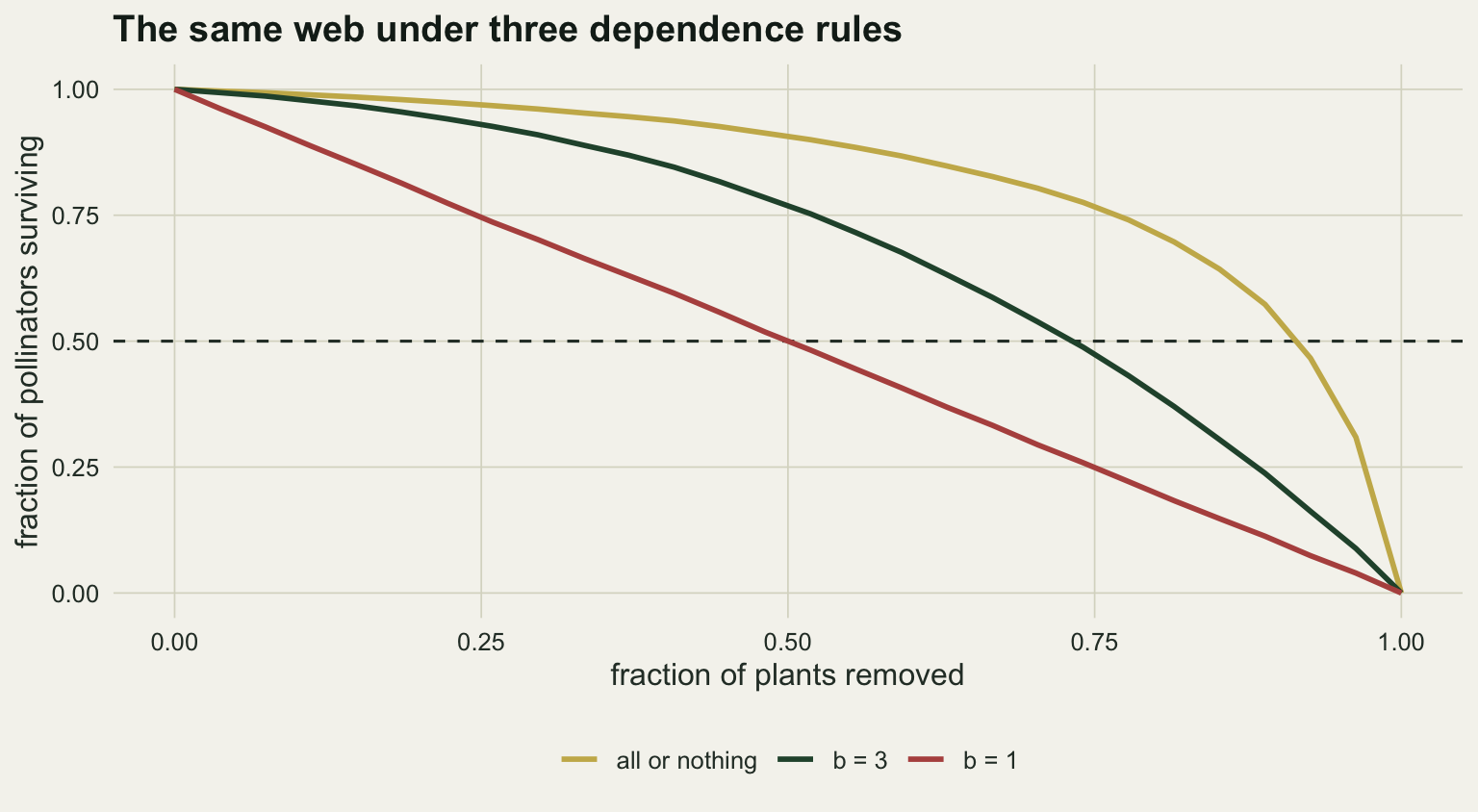
Random removal with the all-or-nothing rule gives R50 0.89, the same number as the section above because it is the same order set. The linear rule on the same web, the same orders and the same thresholds gives 0.49, almost exactly one half, a paired fall of 0.40 with a Monte Carlo standard error of 0.004. That fall is 91 per cent of the distance between most connected first and random on this web, and it is wider than the entire between-web spread under random removal on the fifteen-web bank, 0.11. It comes from an assumption most papers never state, because it is the software default.
The two published results already in the reference list of this post disagree on the sign of the same relationship for the same reason. Dunne et al (2002) report that robustness rises with connectance under the topological rule; Vieira and Almeida-Neto (2015) report that it falls with connectance under a stochastic dependence rule. Neither is wrong. They are measuring different quantities and calling both robustness.
None of the rules is the true one. The point is the direction of the error. The topological curve is the most optimistic curve any dependence rule can produce, so it is an upper bound on persistence rather than an estimate of it, and reporting it as though it were an estimate builds the optimism into the conclusion.
Rewiring, and the two errors that do not cancel
There is an error running the other way, and nothing here measures it. The simulation will not let a pollinator visit a plant it was never recorded on. A bumblebee whose main forage plant has gone does not sit and starve beside a flowering patch it did not happen to use during the sampling; it switches. Kaiser-Bunbury et al (2010) built pollination cascades that allow that switching, and letting pollinators rewire lifts the curves above the fixed-topology version of the same web.
So the accounting holds an overstatement and an understatement at once, and there is no basis for hoping they cancel. They act on different species: rewiring rescues the generalists, which are the species least likely to be stranded in the first place, while the dependence rule bites hardest on the partly depleted specialists that the topological rule scores as perfectly healthy. One is set by foraging flexibility and the other by tolerance of reduced resources, and the output cannot tell you whether they happened to offset.
Honest limits
Observed degree is a function of sampling effort. A plant recorded with two visitors may have twenty, so a thinly sampled web arrives carrying manufactured specialists, and those are the species stranded first in any of these simulations. Effort is rarely even across species within a web, so the bias does not cancel when webs are compared. Checking a network analysis covers the effort sensitivity in more detail.
Fifteen simulated webs are not a sample of real ones. The four generators span connectance 0.20 to 0.53 and plant-degree variation from almost none to a coefficient of variation of 1.00, which is wider than the generator’s own three webs and neither obviously wider nor obviously narrower than the published literature. The bank supports a qualitative claim: webs that differ in topology as well as in parameters separate on R50 by more than the removal order does within any one of them. It cannot support a number for how much more, and the ordering would not survive a bank restricted to webs with strongly uneven plant degrees, which is where a degree-based order has most to exploit.
R50 on a small web is coarse. With 27 plants the survivor fraction can only take 37 values and the removed fraction 28, so the crossing point is interpolated between steps of 0.037. Two webs whose R50 differ by less than a step or two are not distinguishable on this statistic, and the between-web spread under random removal is only about 2.9 steps wide on a web this size. That is wide enough to say the rule effect above is larger, and too narrow to sit in the denominator of a ratio.
Robustness here is also a different quantity from the dynamical stability that May’s work is about, and the two get conflated in discussion. Species are deleted, links are recounted, nobody has a population size and nothing is integrated forward in time; that side of the argument is worked through in stability and complexity in food webs.
Finally, the stochastic rule has no more empirical backing than the all-or-nothing one. It is a demonstration that the choice matters, not a recommendation of an exponent. R50 is not a property of a network that travels between studies. It is a property of the web, the order and the rule together, and a number quoted without the last two cannot be read.
References
Memmott J, Waser NM, Price MV 2004 Proceedings of the Royal Society B 271(1557):2605-2611 (10.1098/rspb.2004.2909)
Dunne JA, Williams RJ, Martinez ND 2002 Ecology Letters 5(4):558-567 (10.1046/j.1461-0248.2002.00354.x)
Burgos E, Ceva H, Perazzo RPJ, Devoto M, Medan D, Zimmermann M, Delbue AM 2007 Journal of Theoretical Biology 249(2):307-313 (10.1016/j.jtbi.2007.07.030)
Kaiser-Bunbury CN, Muff S, Memmott J, Muller CB, Caflisch A 2010 Ecology Letters 13(4):442-452 (10.1111/j.1461-0248.2009.01437.x)
Vieira MC, Almeida-Neto M 2015 Ecology Letters 18(2):144-152 (10.1111/ele.12394)