niche_web <- function(S, C) {
  n <- runif(S)                     # niche value: a position on the feeding axis
  beta <- 1 / (2 * C) - 1           # sets mean range width to hit connectance C
  r <- n * rbeta(S, 1, beta)        # feeding range, always at most the niche value
  r[which.min(n)] <- 0              # smallest niche eats nothing: a basal resource
  centre <- runif(S, r / 2, n)      # range centre, placed below the niche value
  A <- matrix(0L, S, S)
  for (i in seq_len(S)) {
    lo <- centre[i] - r[i] / 2
    hi <- centre[i] + r[i] / 2
    A[i, n >= lo & n <= hi] <- 1L   # eat everything whose niche is inside the range
  }
  A
}
The niche model of food webs
R
food webs
ecological networks
community ecology
ecology tutorial
The niche model of food webs in R, compared with the cascade and random models: one feeding axis reproduces real structure, while a random graph does not.
Corrected 30 September 2026: the post said the niche model produces far more cannibalism than real webs and read its undefined trophic levels as feeding loops; it now says that the post made no such comparison, that the model’s authors report it predicts the degree of cannibalism in real webs, and that the undefined trophic levels come almost entirely from species that eat only themselves.
The previous post measured a food web that was written down by hand. This one asks where such structure comes from. Given only the number of species and the connectance, can a simple rule generate a web that looks like the real thing: the right mix of plants, herbivores and predators, chains of a believable length, a scatter of omnivores? The niche model of Williams and Martinez says yes, and it needs a single idea: lay every species on one feeding axis, and let each one eat a contiguous slice of it. This post builds the model in base R, draws a web from it, and pits it against two older models to show what “realistic” actually buys you.
One axis, one rule
Give every species a niche value between 0 and 1, a position on an abstract feeding axis (loosely, body size or some other ordering of who can eat whom). Each species eats every species whose niche value falls inside a feeding range: an interval placed at or below its own value. Two parameters control a range: its width, drawn so that the average width delivers the connectance you asked for, and its centre, placed below the species’ niche value so that a consumer mostly eats smaller things. One species, the one with the lowest niche value, is forced to eat nothing. That single rule makes it a basal resource and roots the whole web.
The beta line is the only piece of arithmetic that matters. The feeding range is the niche value times a Beta random number with mean 1 / (1 + beta); setting beta = 1 / (2C) - 1 makes that mean equal to 2C, which works out so the expected number of links is C times the number of possible links. You ask for a connectance and the model delivers it on average, without any tuning.
set.seed(43)
S <- 30
A <- niche_web(S, 0.15)

gen <- rowSums(A); vul <- colSums(A)
c(species      = S,
  links        = sum(A),
  connectance  = round(sum(A) / S^2, 3),
  basal        = sum(gen == 0),
  intermediate = sum(gen > 0 & vul > 0),
  top          = sum(gen > 0 & vul == 0),
  cannibals    = sum(diag(A)))
species links connectance basal intermediate top
30.000 137.000 0.152 7.000 18.000 5.000
cannibals
5.000 This draw has 7 basal species, 18 intermediate and 5 top, at a connectance of 0.152, close to the 0.15 requested. It also has 5 cannibals: species that eat their own kind, which the model allows whenever a feeding range covers a species’ own niche value. Real webs have some cannibalism too, and we will come back to that.
library(ggplot2)

# recover the ranges for the drawn web by rerunning with the same seed
set.seed(43)
n <- runif(S); beta <- 1 / (2 * 0.15) - 1; r <- n * rbeta(S, 1, beta)
r[which.min(n)] <- 0; centre <- runif(S, r / 2, n)

ord <- order(n)
df <- data.frame(niche = n[ord], lo = (centre - r / 2)[ord],
                 hi = (centre + r / 2)[ord], rank = seq_len(S))
df$role <- ifelse(rowSums(A)[ord] == 0, "basal",
           ifelse(colSums(A)[ord] == 0, "top", "intermediate"))

ggplot(df, aes(y = rank)) +
  geom_segment(aes(x = lo, xend = hi, yend = rank, colour = role), linewidth = 1.6,
               alpha = 0.5) +
  geom_point(aes(x = niche, colour = role), size = 2) +
  scale_colour_manual(values = c(basal = "#4c9f70", intermediate = "#e0c341",
                                 top = "#c1523f")) +
  labs(x = "Niche value", y = "Species (ordered by niche value)", colour = NULL) +
  theme_minimal(base_size = 12) +
  theme(panel.grid.minor = element_blank(),
        legend.position = "top",
        plot.background = element_rect(fill = "#f5f4ee", colour = NA),
        panel.background = element_rect(fill = "#f5f4ee", colour = NA))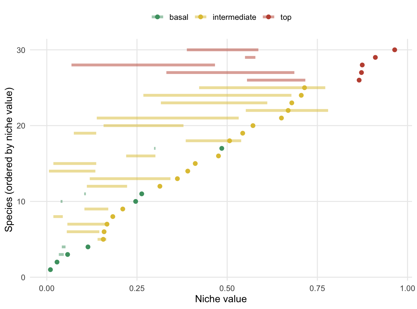
Three models, same connectance
The niche model is one of three classic generators, and the differences between them are the whole point. The random model (an Erdos-Renyi directed graph) fills the whole matrix with links at probability C, ignoring any ordering. The cascade model gives species a rank and lets a consumer eat only lower-ranked species, so the web is strictly hierarchical with no loops. The niche model keeps the ordering of the cascade but replaces “eat anything below you” with “eat a contiguous interval”, which is what lets it produce omnivores, cannibals and the occasional loop.
cascade_web <- function(S, C) {
  p <- 2 * C * S / (S - 1)          # link probability that matches connectance C
  A <- matrix(0L, S, S)
  for (i in 2:S) for (j in 1:(i - 1)) if (runif(1) < p) A[i, j] <- 1L
  A
}
random_web <- function(S, C) matrix(rbinom(S * S, 1, C), S, S)

troph <- function(A) {              # prey-averaged trophic level, or NA if undefined
  S <- nrow(A); W <- A / pmax(rowSums(A), 1)
  tryCatch(solve(diag(S) - W, rep(1, S)), error = function(e) rep(NA_real_, S))
}

props <- function(f, S = 30, C = 0.15, reps = 1000) {
  z <- t(replicate(reps, {
    A <- f(S, C); g <- rowSums(A); v <- colSums(A); tl <- troph(A)
    c(connectance = sum(A) / S^2,
      no_basal    = sum(g == 0) == 0,
      basal_frac  = mean(g == 0),
      tl_undef    = any(!is.finite(tl)) | any(tl > 100))
  }))
  colMeans(z)
}

set.seed(2024)
summ <- rbind(niche   = props(niche_web),
              cascade = props(cascade_web),
              random  = props(random_web))
round(summ, 3)
connectance no_basal basal_frac tl_undef
niche 0.151 0.000 0.207 0.354
cascade 0.150 0.000 0.105 0.000
random 0.150 0.786 0.008 0.807Every model hits the target connectance: the realised values are all near 0.15. What separates them is whether the web they build is a web at all. Look at the no_basal column, the fraction of generated webs with no basal species. For the niche and cascade models it is 0: every web has a producer. For the random model it is 0.786. At a connectance typical of real food webs, a random graph of 30 species leaves every single species eating something about four times in five, so there is no bottom to the web and no energy source. It is not a worse food web; most of the time it is not a food web.
nb <- data.frame(model = rownames(summ), no_basal = summ[, "no_basal"])
nb$model <- factor(nb$model, levels = c("niche", "cascade", "random"))

ggplot(nb, aes(model, no_basal, fill = model)) +
  geom_col(width = 0.6) +
  scale_fill_manual(values = c(niche = "#4c9f70", cascade = "#3d6cb0",
                               random = "#c1523f"), guide = "none") +
  labs(x = NULL, y = "Fraction of webs with no basal species") +
  ylim(0, 1) +
  theme_minimal(base_size = 12) +
  theme(panel.grid.minor = element_blank(),
        panel.grid.major.x = element_blank(),
        plot.background = element_rect(fill = "#f5f4ee", colour = NA),
        panel.background = element_rect(fill = "#f5f4ee", colour = NA))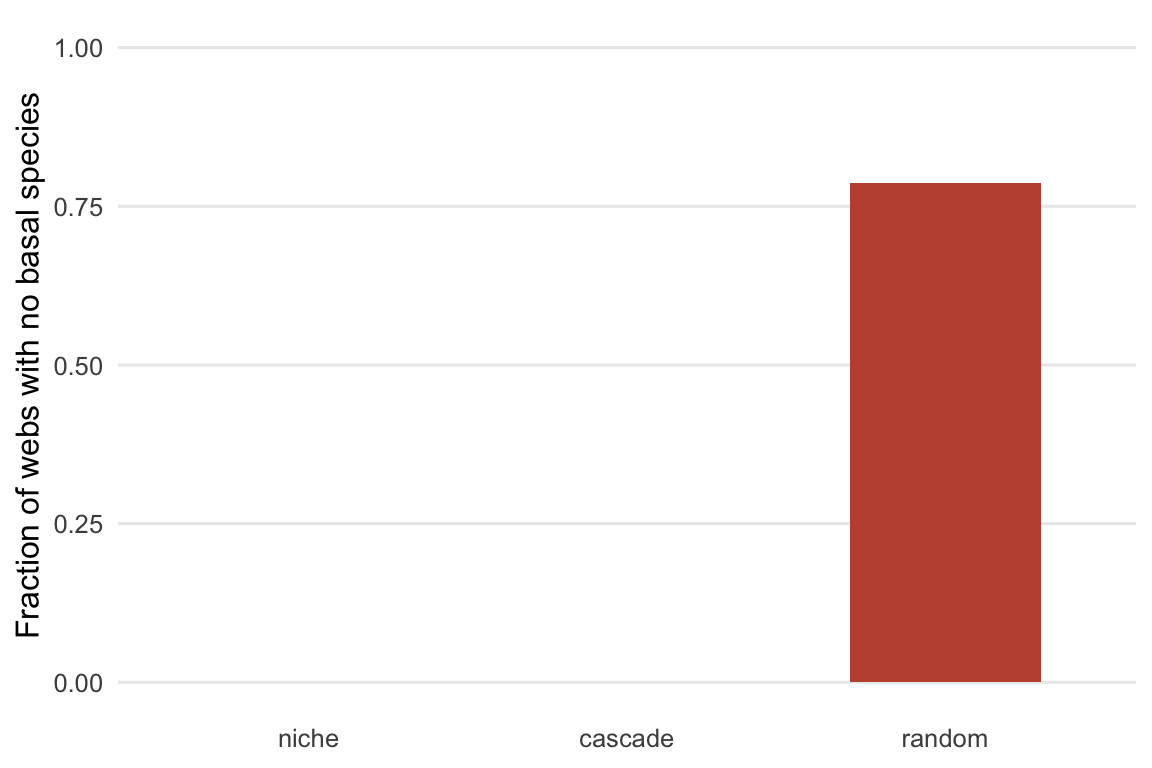
The mean basal fraction tells the same story from the other side. The niche model puts about 21% of species at the base, in the range real webs show. The cascade model roots the web too but keeps fewer species basal, around 11%. The random model averages under 1%: not just often unrooted, but structurally top-heavy in a way no real community is.
What the model gets wrong
None of this makes the niche model true. It is a null model for structure, not a mechanism: it says nothing about who actually eats whom, only that if you assume one feeding axis and interval diets, the coarse counts come out right. Two caveats are worth stating plainly. First, cannibalism: the example web had 5 self-eaters, because nothing stops a feeding range from covering its owner’s niche value. This post has not compared that with real webs, and Williams and Martinez (2000) report that the niche model predicts the degree of cannibalism in the real webs they tested. Second, species that eat only themselves. At this connectance about 35% of niche webs leave the prey-averaged trophic level undefined. Almost always the cause is a species whose feeding range covers only its own niche value, so it eats nothing but itself and has no route down to a basal species. No real consumer lives on its own kind alone. The cascade model, being strictly hierarchical, never leaves the trophic level undefined: its tl_undef is 0. That is the trade. The cascade model is cleaner but rigid; the niche model is messier, allowing the omnivory and loops that real webs contain but also species that feed only on themselves.
So the niche model earns its place not by being right but by being the simplest rule that fails in interesting ways. A random graph fails boringly, by not making a web. The niche model makes a web and then makes the same kinds of mistakes a real web does. That is why it became the baseline against which structural claims are tested, and why the next post can ask a sharper question: given a web with this structure, is it stable?
Where to go next
The connectance and trophic level post defines the roles and measures used here. The next post, stability and complexity, takes a web of a given size and connectance and asks whether it can persist. For the general machinery of testing observed structure against a generated baseline, see null models for interaction networks.
References
Williams RJ, Martinez ND 2000 Nature 404(6774):180-183 (10.1038/35004572)
Cohen JE, Newman CM 1985 Proceedings of the Royal Society of London B 224(1237):421-448 (10.1098/rspb.1985.0042)
Williams RJ, Martinez ND 2004 American Naturalist 163(3):458-468 (10.1086/381964)
Dunne JA, Williams RJ, Martinez ND 2002 Proceedings of the National Academy of Sciences 99(20):12917-12922 (10.1073/pnas.192407699)