---
title: "Diet choice and the zero-one rule"
description: "The prey model in R: rank prey by profitability, the zero-one rule, and why a poor prey's place in the diet depends only on how common the good prey are."
date: "2026-06-30 12:00"
date-modified: "2026-10-15"
categories: [ecology tutorial, R, foraging, behaviour, species interactions]
image: thumbnail.png
image-alt: "A grid of good and poor prey abundances shaded by whether the poor prey is eaten, with a vertical boundary showing it depends only on the good prey."
---
*Corrected 15 October 2026: the introduction said searching costs the chance of meeting a better item; it now says that chance is what attacking gives up during handling, and that ignoring an item costs the energy it would have given.*
```{r setup}
#| code-fold: true
#| code-summary: "Setup: packages, colours and plot theme"
#| results: hide
#| message: false
#| warning: false
knitr::opts_chunk$set(echo = TRUE, message = FALSE, warning = FALSE,
                      dev = "png", dpi = 120, fig.path = "figures/",
                      fig.width = 7, fig.height = 4.4)
library(ggplot2)
theme_te <- theme_minimal(base_size = 12) +
  theme(panel.background = element_rect(fill = "#f5f4ee", colour = NA),
        plot.background  = element_rect(fill = "#f5f4ee", colour = NA),
        panel.grid.minor = element_blank(),
        plot.title = element_text(face = "bold", size = 12))
theme_set(theme_te)
col_in <- "#3a6b52"; col_out <- "#b5651d"; col_ref <- "#555555"

## two prey types: 1 profitable, 2 poor
e1 <- 8; h1 <- 1; e2 <- 2; h2 <- 1
prof1 <- e1/h1; prof2 <- e2/h2
rate_only1 <- function(l1) l1*e1 / (1 + l1*h1)
include2   <- function(l1) prof2 > rate_only1(l1)          # l2 does not appear
l1_star    <- prof2 / (e1 - h1*prof2)                       # threshold in good-prey encounter rate
```
A predator meets prey one at a time and, on each encounter, makes a choice: attack this one, or ignore it and keep searching for something better. Attacking costs handling time, during which the forager cannot meet a better item; ignoring costs the energy of the item passed up. The prey model of optimal foraging works out which prey types are worth attacking, and its answer has a sharp, testable edge (MacArthur and Pianka 1966 The American Naturalist 100(916):603-609; Charnov 1976 The American Naturalist 110(971):141-151).
## Profitability and the ranking
Each prey type carries an energy `e`, a handling time `h`, and an encounter rate `lambda` (how often the forager meets it while searching). The key quantity is **profitability**, energy per unit handling time, `e/h`: how much a prey item is worth once you have decided to deal with it. Rank the prey types by profitability, most profitable first, and the optimal diet is built by adding types down the ranking.
```{r profit}
e1 <- 8; h1 <- 1     # profitable prey
e2 <- 2; h2 <- 1     # poor prey
c(profitability_1 = e1/h1, profitability_2 = e2/h2)
```
Include the top type always. Then include the next type only if its profitability is higher than the intake rate you already get from the types above it. For the second type that rate, when the forager takes only type 1, is `lambda_1 e_1 / (1 + lambda_1 h_1)`. Attack the poor prey when
$$\frac{e_2}{h_2} > \frac{\lambda_1 e_1}{1 + \lambda_1 h_1}.$$
## The zero-one rule
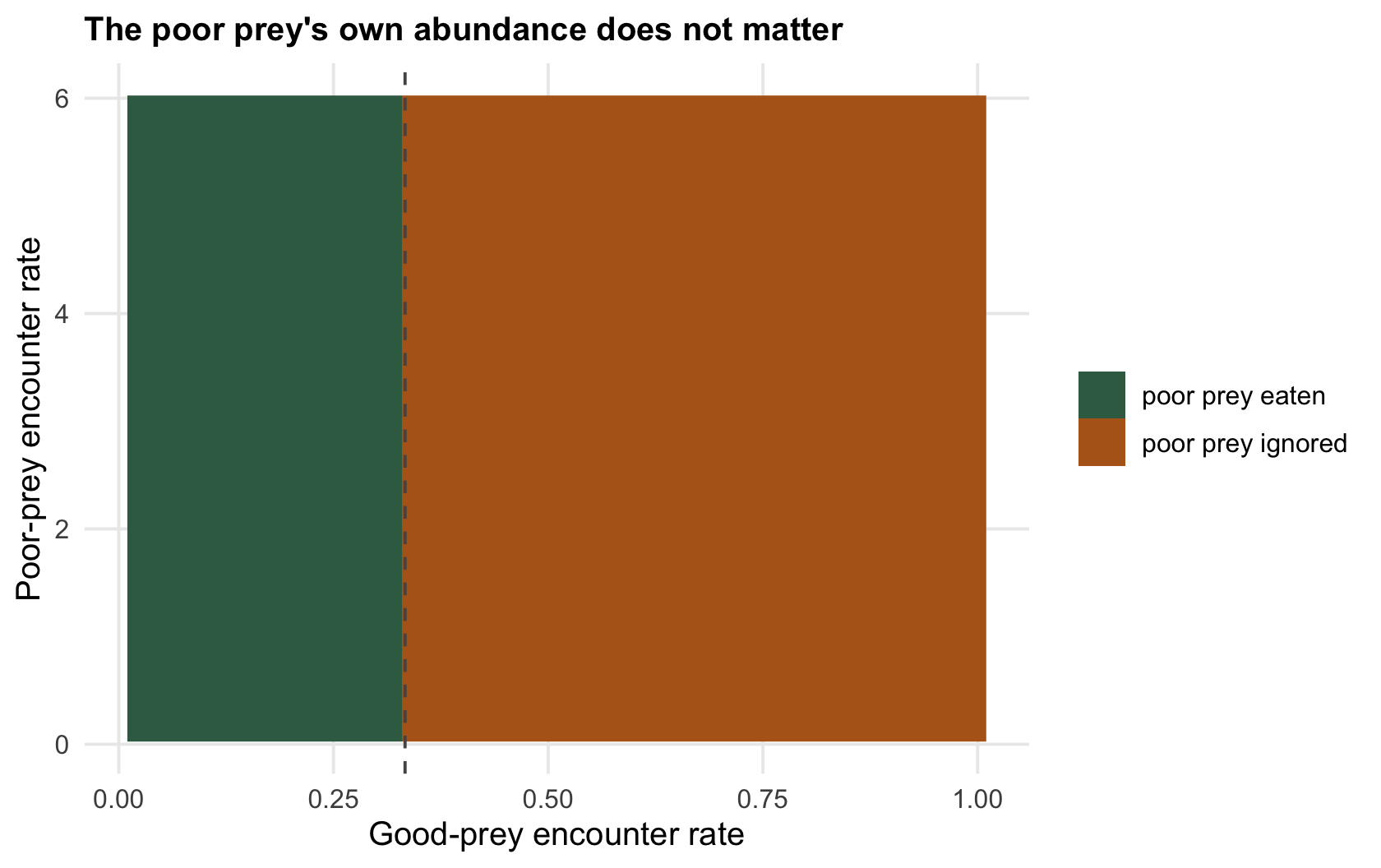
Look hard at that inequality. Its right side does not contain `lambda_2`, the encounter rate of the poor prey itself. Whether the poor prey belongs in the diet is decided entirely by how often the forager meets the *good* prey. This is the zero-one rule: a prey type is either always attacked on encounter or never attacked; there are no partial preferences, and a type's own abundance does not decide its membership.
```{r zero-one}
rate_only1 <- function(l1) l1*e1 / (1 + l1*h1)
include2   <- function(l1, l2) (e2/h2) > rate_only1(l1)    # note: l2 is ignored
# vary the POOR prey abundance, hold the good prey fixed
sapply(c(0.1, 1, 5, 20), function(l2) include2(l1 = 0.2, l2 = l2))
```
Make the poor prey ten times, a hundred times more common, and the answer never changes: at this abundance of the good prey it stays on the menu, no matter how the poor prey swarms. Now move the good prey instead.
```{r vary-good}
sapply(c(0.10, 0.30, 0.34, 1.0), function(l1) include2(l1 = l1, l2 = 5))
```
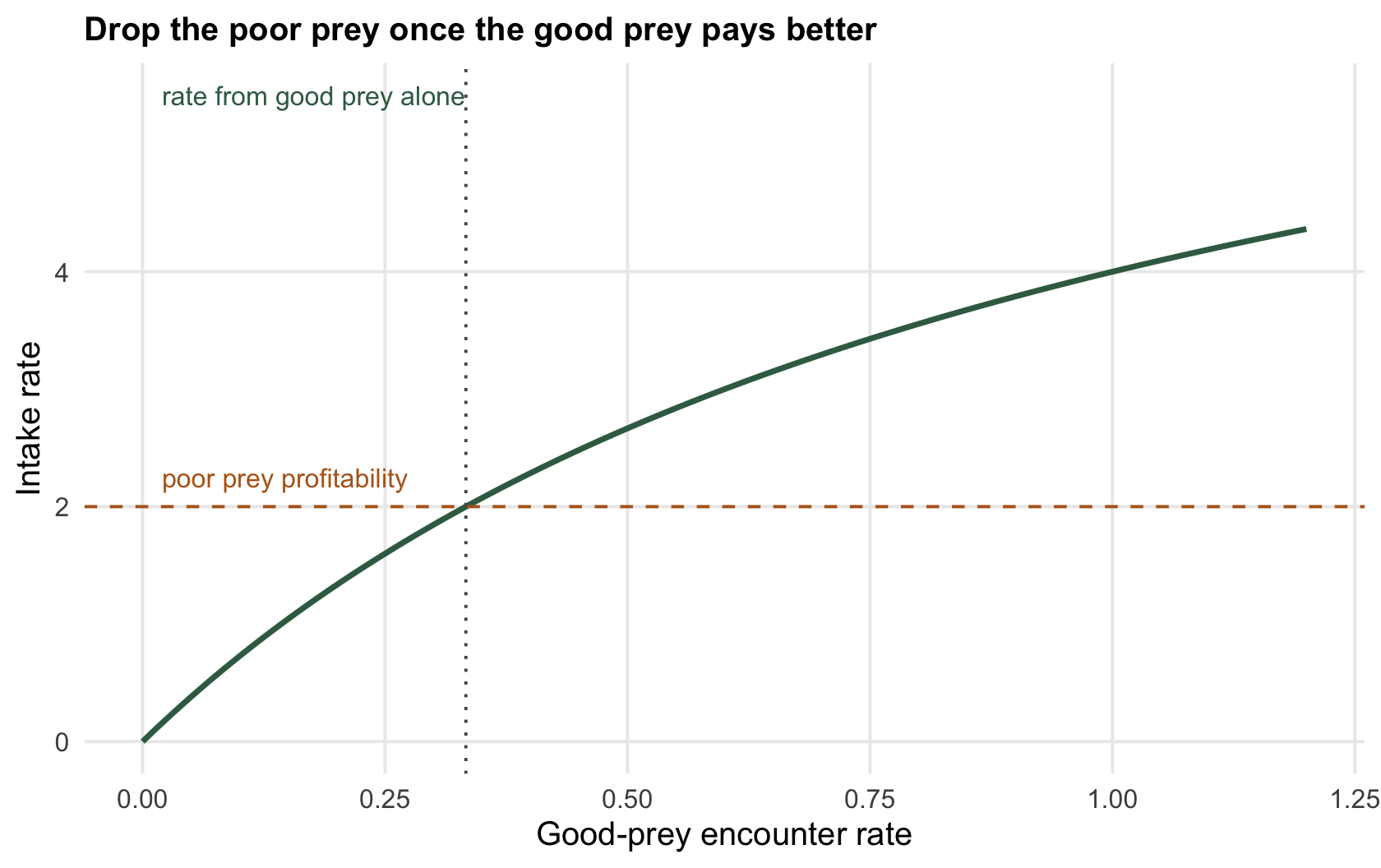
The poor prey is on the menu while the good prey is scarce and drops off it once the good prey passes an encounter rate of `r sprintf("%.2f", l1_star)`. That threshold is where the rate from eating only the good prey rises to equal the poor prey's profitability: below it the poor prey is worth stopping for, above it the forager does better to walk past and hold out for another good item.
```{r fig-grid}
#| fig-cap: "Whether the poor prey is eaten, across abundances of both prey. The boundary is vertical: it depends only on the good prey's encounter rate, never on the poor prey's own."
#| fig-alt: "A shaded grid of good-prey against poor-prey encounter rate; the eaten and ignored regions are split by a vertical line, showing the poor prey's own abundance is irrelevant."
gr <- expand.grid(l1 = seq(0.02, 1, 0.02), l2 = seq(0.1, 6, 0.15))
gr$eaten <- ifelse((e2/h2) > gr$l1*e1/(1 + gr$l1*h1), "poor prey eaten", "poor prey ignored")
ggplot(gr, aes(l1, l2, fill = eaten)) +
  geom_raster() +
  geom_vline(xintercept = l1_star, colour = col_ref, linetype = "dashed") +
  scale_fill_manual(values = c("poor prey eaten" = col_in, "poor prey ignored" = col_out)) +
  labs(x = "Good-prey encounter rate", y = "Poor-prey encounter rate", fill = NULL,
       title = "The poor prey's own abundance does not matter")
```
## Become choosier when times are good
The rule inverts a natural expectation. You might think a forager surrounded by poor prey would eat them, if only for want of anything better. It does, but only while the good prey is rare. As the good prey becomes abundant the forager should become *more* selective and refuse the poor prey, even as the poor prey grows more common underfoot. Selectivity tracks the richness of the good option, not the scarcity of food in general.
```{r fig-switch}
#| fig-cap: "The decision as the good prey becomes common. While the rate from the good prey alone (green) is below the poor prey's profitability (dashed), the poor prey is worth taking; past the crossover the forager should ignore it."
#| fig-alt: "A rising curve of intake rate from the good prey alone crossing a horizontal line marking the poor prey's profitability; left of the crossing the poor prey is eaten, right of it ignored."
l1g <- seq(0, 1.2, 0.01)
dd <- data.frame(l1 = l1g, rate1 = rate_only1(l1g))
ggplot(dd, aes(l1, rate1)) +
  geom_line(colour = col_in, linewidth = 1) +
  geom_hline(yintercept = e2/h2, colour = col_out, linetype = "dashed") +
  geom_vline(xintercept = l1_star, colour = col_ref, linetype = "dotted") +
  annotate("text", x = 0.02, y = e2/h2 + 0.25, label = "poor prey profitability", hjust = 0, colour = col_out, size = 3.4) +
  annotate("text", x = 0.02, y = 5.5, label = "rate from good prey alone", hjust = 0, colour = col_in, size = 3.4) +
  labs(x = "Good-prey encounter rate", y = "Intake rate",
       title = "Drop the poor prey once the good prey pays better")
```
## What the model leaves out
The prey model is a clean idealisation, and its cleanliness is also its limit. It assumes the forager recognises prey instantly and perfectly, encounters them one at a time and at random, and is paid in long-run intake rate. Real foragers sample, learn, mistake one prey for another, and often show *partial* preferences, taking a poor prey on some encounters and not others, exactly what the zero-one rule forbids. Those partial preferences are not a failure of the theory so much as a measurement of what the theory omits: recognition time, incomplete information, nutrient balancing, the risk of being eaten while choosy. The [checking post](../checking-a-foraging-analysis/) takes up which currency a forager is really counting, and the posts on either side of this one cover the other half of the foraging problem: [when to leave a patch](../the-marginal-value-theorem/) and [how fast a predator eats](../functional-responses-holling/).
## References
- Charnov EL 1976. The American Naturalist 110(971):141-151 (10.1086/283054).
- MacArthur RH, Pianka ER 1966. The American Naturalist 100(916):603-609 (10.1086/282454).
- Pyke GH 1984. Annual Review of Ecology and Systematics 15(1):523-575 (10.1146/annurev.es.15.110184.002515).
## Related tutorials
- [Functional responses in R](../functional-responses-holling/)
- [The marginal value theorem](../the-marginal-value-theorem/)
- [Checking a foraging analysis](../checking-a-foraging-analysis/)
- [Patch-leaving rules and prey clumping](../patch-leaving-rules-and-prey-clumping/)