library(ggplot2)

te_paper  <- "#f5f4ee"
te_ink    <- "#16241d"
te_body   <- "#2c3a31"
te_forest <- "#275139"
te_rust   <- "#b5534e"
te_gold   <- "#c9b458"
te_line   <- "#dad9ca"

theme_datasheet <- function() {
  theme_minimal(base_size = 12) +
    theme(plot.background  = element_rect(fill = te_paper, colour = NA),
          panel.background = element_rect(fill = te_paper, colour = NA),
          panel.grid.major = element_line(colour = te_line, linewidth = 0.3),
          panel.grid.minor = element_blank(),
          text             = element_text(colour = te_body),
          plot.title       = element_text(colour = te_ink, face = "bold"),
          plot.subtitle    = element_text(colour = te_body),
          axis.text        = element_text(colour = te_body))
}Patch-leaving rules and prey clumping
R
foraging
behaviour
simulation
ecology tutorial
Fixed number, fixed time or giving-up time: which patch-leaving rule pays depends on how prey are spread among patches. Measured in R for a blind forager.
A parasitoid wasp lands on a leaf and starts searching for aphids. It cannot see how many aphids the leaf holds; it only finds out one aphid at a time, as it bumps into them. Some leaves carry a colony of forty, many carry none, and a few carry two or three. At some point the wasp flies to another leaf, and the flight costs time that finds nothing. The question is what it should use to decide when to go: the time it has spent on the leaf, the number of aphids it has already found, or the time since it last found one.
The marginal value theorem (Charnov 1976) answers a neighbouring question. It gives the forager a known, smooth gain curve for the patch and finds the residence time at which the marginal rate falls to the long-run rate. Its closing section, “What the theorem assumes”, says that real animals use rules of thumb instead, leaving “when the capture rate drops below a threshold, or after a fixed unrewarded interval”, and that these approximate the theorem well. This post puts numbers on those rules of thumb for a forager that cannot see the gain curve of the patch it is in, and the numbers do not single out one rule: which rule does well depends on how prey are distributed among patches. The checking post for foraging analyses asks which currency the animal is counting and whether prey deplete during a trial; here the currency is fixed as the long-run intake rate, depletion is built in, and the thing that varies is the spread of prey among patches.
The result is not new. Iwasa, Higashi and Yamamura (1981) set out exactly this comparison: three elementary rules, each with its one parameter optimised, and a ranking that “depends critically on the type of prey distribution between patches”. What the post adds is a version you can run, the numbers for one parameter set, a check of the two exact results the paper gives, and the amount of clumping at which a giving-up-time rule starts to beat a fixed residence time, which turns out to move with travel time.
A forager that finds prey one at a time
The search model is random search. A patch holds n prey, and while m of them remain the forager finds the next one after an exponential waiting time with rate a times m. That is the same as saying that each prey item is found at its own exponential time with rate a, independently of the others, and it is the random search assumption Iwasa and colleagues work under (their paper frames the model as stochastic and discrete; the version here uses continuous exponential waiting times). Handling time is zero, so intake is the number of prey found. Between patches the forager travels for a fixed time that yields nothing, and the prey count of the next patch is a fresh draw from the between-patch distribution, which the forager knows. It does not know the count of the patch it is in.
Three elementary rules are compared. The fixed-time rule leaves after a residence time T. The giving-up-time rule leaves once an interval G passes with no capture, counting from arrival or from the last capture. The fixed-number rule leaves after its k-th capture; because a patch can hold fewer than k prey, that rule on its own can wait forever, so it carries a time cap C as well and leaves at whichever comes first. The number rule therefore has two parameters, and with k larger than any patch it becomes the fixed-time rule, which matters for reading its results.
Every rule is scored by the same currency, the long-run intake rate: total prey found divided by total time, residence plus travel, over a long sequence of patches. Each rule’s parameter is chosen by a fine grid search on one set of 20000 simulated patches and its rate is then measured on an independent set of the same size, and the two sets swap roles. Choosing and scoring on the same patches would reward the rule with more freedom to fit noise. The curves are computed from sorted capture times rather than by looping over patches, which keeps each grid search to a fraction of a second.
mean_prey <- 5
a_rate    <- 0.3
tau_main  <- 2
n_patch   <- 20000

make_patches <- function(n_vec) {
  n_max <- max(n_vec, 1)
  m     <- length(n_vec)
  left  <- outer(n_vec, 0:(n_max - 1), "-")
  gaps  <- matrix(rexp(m * n_max), m) / (a_rate * pmax(left, 1))
  gaps[left <= 0] <- Inf
  cum <- gaps
  if (n_max > 1) for (j in 2:n_max) cum[, j] <- cum[, j - 1] + gaps[, j]
  list(n = n_vec, gaps = gaps, cum = cum, m = m)
}

time_curve <- function(p, t_vals, tau) {
  key <- sort(p$cum[is.finite(p$cum)])
  findInterval(t_vals, key) / (p$m * (t_vals + tau))
}

gut_curve <- function(p, g_vals, tau) {
  run_max <- p$gaps
  if (ncol(run_max) > 1)
    for (j in 2:ncol(run_max)) run_max[, j] <- pmax(run_max[, j - 1], run_max[, j])
  ok   <- is.finite(run_max)
  ord  <- order(run_max[ok])
  key  <- run_max[ok][ord]
  gsum <- c(0, cumsum(p$gaps[ok][ord]))
  idx  <- findInterval(g_vals, key)
  idx / (gsum[idx + 1] + p$m * (g_vals + tau))
}

number_surface <- function(p, k_vals, c_vals, tau) {
  n_col  <- ncol(p$cum)
  gain_k <- matrix(0, n_col + 1, length(c_vals))
  time_k <- matrix(0, n_col + 1, length(c_vals))
  run_gain <- 0
  for (j in seq_len(n_col)) {
    s_j  <- sort(p$cum[, j])
    cs_j <- c(0, cumsum(s_j))
    n_le <- findInterval(c_vals, s_j)
    run_gain    <- run_gain + n_le
    gain_k[j, ] <- run_gain
    time_k[j, ] <- cs_j[n_le + 1] + (p$m - n_le) * c_vals
  }
  gain_k[n_col + 1, ] <- run_gain
  time_k[n_col + 1, ] <- p$m * c_vals
  k_use <- pmin(k_vals, n_col + 1)
  gain_k[k_use, , drop = FALSE] /
    (time_k[k_use, , drop = FALSE] + p$m * tau)
}

t_vals <- seq(0.05, 20, by = 0.05)
g_vals <- seq(0.05, 15, by = 0.025)
k_vals <- 1:60
c_vals <- seq(0.25, 20, by = 0.25)

exact_time <- function(tau) mean_prey * (1 - exp(-a_rate * t_vals)) / (t_vals + tau)
t_star     <- t_vals[which.max(exact_time(tau_main))]
rate_star  <- max(exact_time(tau_main))

set.seed(4127)
chk_pois <- make_patches(rpois(n_patch, mean_prey))
chk_nb   <- make_patches(rnbinom(n_patch, mu = mean_prey, size = 0.5))
sim_at_star <- c(time_curve(chk_pois, t_star, tau_main),
                 time_curve(chk_nb, t_star, tau_main))
se_at_star  <- c(sd(rowSums(chk_pois$cum <= t_star)),
                 sd(rowSums(chk_nb$cum <= t_star))) / sqrt(n_patch) / (t_star + tau_main)
z_at_star   <- (sim_at_star - rate_star) / se_at_star
chk_nest <- max(abs(number_surface(chk_nb, max(chk_nb$n) + 1, c_vals, tau_main) -
                    time_curve(chk_nb, c_vals, tau_main)))
The design constants were fixed before anything ran: a mean of 5 prey per patch, a search rate of 0.3 per prey item per unit time, and a travel time of 2 time units. They match a pilot run of the same comparison and were not revised afterwards.
One rule has an exact answer that makes a good check on the simulator. Under a fixed residence time T each of the n prey is found by time T with probability one minus exp(-aT), so the expected intake per patch is the mean prey count times that probability whatever the distribution of counts, and the long-run rate is that divided by T plus the travel time. Maximising it on the grid gives T = 3.10 and a rate of 0.5936 prey per unit time. The simulated fixed-time rate at that T is 0.5920 for Poisson patches and 0.5975 for strongly clumped ones, which are -0.6 and 0.6 Monte Carlo standard errors from the exact value. A second check is structural: with k above the largest patch the number rule’s surface should equal the fixed-time curve exactly, and the largest difference is exactly zero.
The fixed-time result also says something before any comparison. A forager on a clock collects the same long-run rate on even, Poisson or clumped patches with the same mean. The distribution can only matter through what the forager learns while it searches.
What a capture says about the prey still in the patch
Iwasa and colleagues show that under random search the number of captures so far, c, and the time spent, t, are all the forager needs: the exact timing of earlier captures adds nothing. The expected number of prey left given c and t has a closed form for the three distributions used here. For an even distribution every patch holds the mean, so the prey left are the mean minus c, whatever the time. For a Poisson distribution the prey left are Poisson with mean mean_prey * exp(-a t), which does not depend on c at all. For a negative binomial distribution with size parameter s, the prey left are negative binomial again, with mean (c + s) z / (1 - z), where z = exp(-a t) times mean_prey / (mean_prey + s); each capture raises the estimate. A size of 0.5 is used below as the clumped case.
t_look  <- 3
c_look  <- 0:10
size_cl <- 0.5
z_look  <- mean_prey / (mean_prey + size_cl) * exp(-a_rate * t_look)

post_df <- rbind(
  data.frame(captures = c_look, left = pmax(mean_prey - c_look, 0), dist = "even"),
  data.frame(captures = c_look, left = mean_prey * exp(-a_rate * t_look), dist = "Poisson"),
  data.frame(captures = c_look, left = (c_look + size_cl) * z_look / (1 - z_look),
             dist = "clumped"))

sim_post <- function(p, lab) {
  caught <- rowSums(p$cum <= t_look)
  agg    <- aggregate(p$n - caught, list(captures = caught), mean)
  n_cell <- tabulate(caught + 1)[agg$captures + 1]
  data.frame(captures = agg$captures, sim_left = agg$x, n_cell = n_cell, dist = lab)
}
post_sim <- rbind(sim_post(chk_pois, "Poisson"), sim_post(chk_nb, "clumped"))
post_sim <- merge(post_sim[post_sim$n_cell >= 200 & post_sim$captures <= 10, ],
                  post_df, by = c("captures", "dist"))
post_gap <- max(abs(post_sim$sim_left - post_sim$left))
sd_cell  <- function(p, lab) {
  caught <- rowSums(p$cum <= t_look)
  agg    <- aggregate(p$n - caught, list(captures = caught), sd)
  data.frame(captures = agg$captures, sd_left = agg$x, dist = lab)
}
post_sim <- merge(post_sim, rbind(sd_cell(chk_pois, "Poisson"), sd_cell(chk_nb, "clumped")),
                  by = c("captures", "dist"))
post_z   <- max(abs(post_sim$sim_left - post_sim$left) / (post_sim$sd_left / sqrt(post_sim$n_cell)))
n_cells  <- nrow(post_sim)

cl_left  <- post_df$left[post_df$dist == "clumped"]
cl_zero  <- cl_left[1]
cl_four  <- cl_left[5]
pois_left <- mean_prey * exp(-a_rate * t_look)
At 3 time units into a visit, close to the optimal fixed residence time, a forager on Poisson patches expects 2.03 prey left whether it has caught none or ten. On clumped patches the same forager expects 0.29 prey left after no captures and 2.64 after four. The patches simulated for the check above agree with the closed forms: across every capture count with at least 200 patches, the largest gap between the simulated mean and the formula is 0.193 prey, and the largest in units of its own standard error is 1.6 over 19 cells.
post_df$dist  <- factor(post_df$dist, levels = c("even", "Poisson", "clumped"))
post_sim$dist <- factor(post_sim$dist, levels = c("even", "Poisson", "clumped"))
ggplot(post_df, aes(captures, left, colour = dist)) +
  geom_line(linewidth = 0.9) +
  geom_point(data = post_sim, aes(y = sim_left), size = 2.2) +
  scale_colour_manual(values = c(even = te_gold, Poisson = te_forest, clumped = te_rust),
                      name = NULL) +
  scale_x_continuous(breaks = 0:10) +
  labs(x = "prey caught so far", y = "expected prey still in the patch",
       title = "A capture is good news only when prey are clumped",
       subtitle = "three time units into the visit; mean of five prey per patch") +
  theme_datasheet() +
  theme(legend.position = "bottom")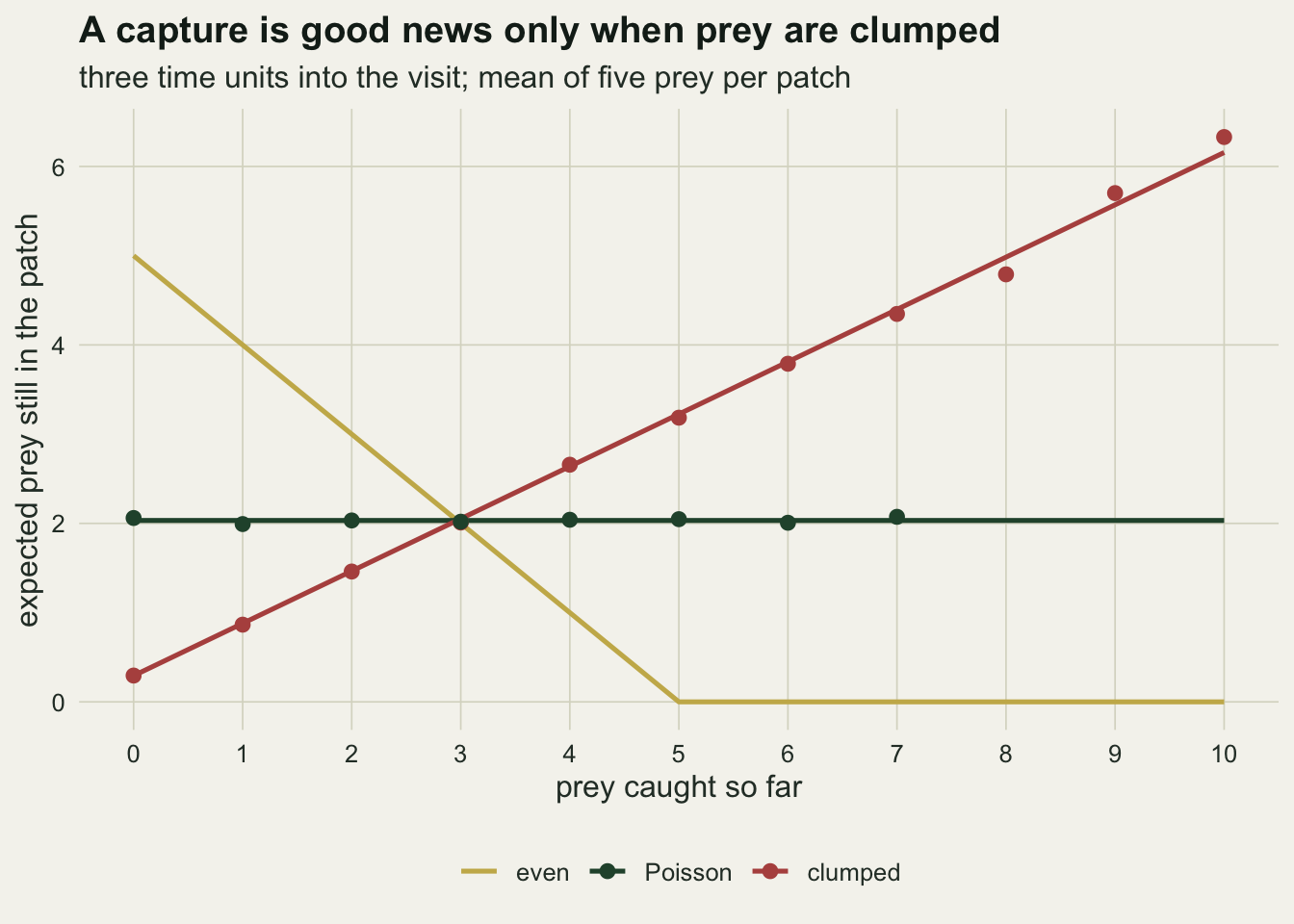
The figure is the whole argument in advance. On even patches a capture means one fewer prey left, so a forager should leave sooner the more it has caught, and counting captures is the natural rule. On Poisson patches a capture carries no information about what is left, so the clock is all the information there is, and Iwasa and colleagues show that the best possible rule then reduces to a fixed residence time. On clumped patches a capture is evidence of a rich patch, so each one should extend the stay, and a giving-up time does that crudely: every capture resets it.
Three distributions, one mean, three different winners
n_rep_rank <- 6
draw_prey <- function(dist, m) switch(dist,
  even    = rep(mean_prey, m),
  Poisson = rpois(m, mean_prey),
  clumped = rnbinom(m, mu = mean_prey, size = size_cl))

bayes_curve <- function(p, h_vals, size, tau) {
  theta <- mean_prey / (mean_prey + size)
  n_col <- ncol(p$cum)
  z     <- theta * exp(-a_rate * p$cum)
  c_mat <- matrix(0:(n_col - 1), p$m, n_col, byrow = TRUE)
  h_mat <- a_rate * (c_mat + size) * z / (1 - z)
  h_mat[!is.finite(p$cum)] <- -Inf
  if (n_col > 1) for (j in 2:n_col) h_mat[, j] <- pmin(h_mat[, j - 1], h_mat[, j])
  cnt_ge <- sapply(seq_len(n_col), function(j)
    p$m - findInterval(h_vals, sort(h_mat[, j]), left.open = TRUE))
  cnt_ge <- cbind(p$m, matrix(cnt_ge, nrow = length(h_vals)))
  cnt_eq <- cnt_ge - cbind(cnt_ge[, -1, drop = FALSE], 0)
  c_all  <- 0:n_col
  vapply(seq_along(h_vals), function(i) {
    w_c <- h_vals[i] / (a_rate * (c_all + size))
    t_c <- pmax(0, log(theta * (1 + w_c) / w_c) / a_rate)
    sum(cnt_eq[i, ] * c_all) / sum(cnt_eq[i, ] * (t_c + tau))
  }, 0)
}
h_vals <- exp(seq(log(0.02), log(4), length.out = 200))

fit_rules <- function(p_train, p_test, dist, tau) {
  t_b  <- t_vals[which.max(time_curve(p_train, t_vals, tau))]
  g_b  <- g_vals[which.max(gut_curve(p_train, g_vals, tau))]
  ns   <- number_surface(p_train, k_vals, c_vals, tau)
  best <- which(ns == max(ns), arr.ind = TRUE)[1, ]
  k_b  <- k_vals[best[1]]
  c_b  <- c_vals[best[2]]
  b_rate <- NA_real_
  if (dist == "clumped") {
    h_b    <- h_vals[which.max(bayes_curve(p_train, h_vals, size_cl, tau))]
    b_rate <- bayes_curve(p_test, h_b, size_cl, tau)
  }
  data.frame(dist = dist,
             time = time_curve(p_test, t_b, tau), t_b = t_b,
             gut = gut_curve(p_test, g_b, tau), g_b = g_b,
             number = number_surface(p_test, k_b, c_b, tau)[1, 1],
             k_b = k_b, c_b = c_b, bayes = b_rate, n_max = max(p_train$n))
}

set.seed(8803)
dist_names <- c("even", "Poisson", "clumped")
rank_raw <- do.call(rbind, lapply(dist_names, function(d) {
  do.call(rbind, lapply(seq_len(n_rep_rank), function(r) {
    p_a <- make_patches(draw_prey(d, n_patch))
    p_b <- make_patches(draw_prey(d, n_patch))
    out <- rbind(fit_rules(p_a, p_b, d, tau_main), fit_rules(p_b, p_a, d, tau_main))
    out$rep <- r
    out
  }))
}))

rep_mean <- aggregate(cbind(time, gut, number, bayes) ~ dist + rep, rank_raw,
                      mean, na.action = na.pass)
rep_mean$gut_minus_time <- rep_mean$gut - rep_mean$time
rep_mean$num_minus_time <- rep_mean$number - rep_mean$time
rank_mean <- aggregate(cbind(time, gut, number, bayes, gut_minus_time, num_minus_time) ~ dist,
                       rep_mean, mean, na.action = na.pass)
rank_se   <- aggregate(cbind(time, gut, number, gut_minus_time, num_minus_time) ~ dist,
                       rep_mean, function(x) sd(x) / sqrt(length(x)))
rownames(rank_mean) <- rank_mean$dist
rownames(rank_se)   <- rank_se$dist

rv <- function(col, d) rank_mean[d, col]
rs <- function(col, d) rank_se[d, col]
k_even   <- range(rank_raw$k_b[rank_raw$dist == "even"])
c_even   <- range(rank_raw$c_b[rank_raw$dist == "even"])
k_pois   <- range(rank_raw$k_b[rank_raw$dist == "Poisson"])
c_pois   <- range(rank_raw$c_b[rank_raw$dist == "Poisson"])
k_clump  <- range(rank_raw$k_b[rank_raw$dist == "clumped"])
c_clump  <- range(rank_raw$c_b[rank_raw$dist == "clumped"])
nmax_cl  <- min(rank_raw$n_max[rank_raw$dist == "clumped"])
cap_pois <- mean_prey * (1 - exp(-a_rate * c_pois[2]))
p_trig   <- ppois(k_pois[1] - 1, cap_pois, lower.tail = FALSE)
t_third  <- sum(1 / (a_rate * (mean_prey:(mean_prey - 2))))
share_cl <- (rv("gut", "clumped") - rv("time", "clumped")) /
            (rv("bayes", "clumped") - rv("time", "clumped"))
z_pois   <- rv("num_minus_time", "Poisson") / rs("num_minus_time", "Poisson")
n_fit    <- 2 * n_rep_rank
ratio_even  <- rv("number", "even") / rv("time", "even")
ratio_clump <- rv("gut", "clumped") / rv("time", "clumped")
bayes_gain  <- rv("bayes", "clumped") / rv("gut", "clumped")
Each distribution was run with 6 independent pairs of patch sets, each pair giving two cross-fitted estimates, so every rate below is a mean over 12 scorings and its Monte Carlo standard error comes from the spread of the 6 pair means.
On even patches, all holding 5 prey, the number rule reaches 0.651 prey per unit time, the fixed-time rule 0.594 and the giving-up-time rule 0.535, with standard errors no larger than 0.0004. The number rule is 1.10 times the fixed-time rate. Its optimum was k = 3 in every scoring, with a cap between 11.50 and 15.00, several times the mean time to the third capture of 2.61: the forager takes the first three prey and leaves the two slow ones behind.
On Poisson patches the fixed-time rule reaches 0.59392 and the number rule 0.59355, a difference of -0.0004 with a standard error of 0.0002, so the two-parameter rule came out 2.5 standard errors below the one-parameter clock, which is consistent with the cost of fitting a second parameter to noise. The optimised number rule set its count between 9 and 13 and its cap between 3.00 and 3.25, and at a cap of 3.25 the catch is Poisson with mean 3.11, so even the smallest of those counts is reached in only 0.0048 of patches and the rule has turned itself into a clock. That is the paper’s Poisson result showing up as an optimiser’s choice: when captures carry no information, a rule that listens to them has nothing to gain. The giving-up-time rule is below both at 0.564. Its departures depend on the chance length of one waiting time, which adds variation in residence time without adding information.
On clumped patches the order reverses. The giving-up-time rule reaches 0.757 against 0.595 for the fixed-time rule, a ratio of 1.27, and the paired difference of 0.161 has a standard error of 0.0008. The number rule, at 0.595, again became the fixed-time rule: its optimal count ran from 48 to 60, near the top of the grid, with the cap doing all the work.
The clumped case also has an informed rule to compare against. The fourth rule in the figure leaves when the expected capture rate, a times the expected prey left from the formula in the previous section, falls below a threshold, and the threshold is optimised in the same train and test scheme. This is the sophisticated strategy of Iwasa and colleagues, leaving when their estimator of the prey left falls below a critical value, with the critical value found by search rather than derived. It reaches 0.790, 1.044 times the giving-up-time rate. Measured from the fixed-time rate, the giving-up time, whose form ignores the negative binomial (only its one parameter was tuned to it), recovers a share of 0.83 of the informed forager’s gain.
rule_labels <- c(time = "fixed time", gut = "giving-up time",
                 number = "fixed number (with cap)", bayes = "informed threshold")
rank_long <- do.call(rbind, lapply(names(rule_labels), function(r) {
  se_r <- if (r == "bayes") {
    tapply(rep_mean$bayes, rep_mean$dist, function(x) sd(x) / sqrt(length(x)))[rank_mean$dist]
  } else rank_se[rank_mean$dist, r]
  data.frame(dist = rank_mean$dist, rule = rule_labels[[r]],
             rate = rank_mean[[r]], se = as.numeric(se_r))
}))
rank_long <- rank_long[!is.na(rank_long$rate), ]
rank_long$dist <- factor(rank_long$dist, levels = dist_names)
rank_long$rule <- factor(rank_long$rule, levels = rev(unname(rule_labels)))

ggplot(rank_long, aes(rate, rule)) +
  geom_vline(xintercept = rate_star, linetype = "dashed", colour = te_body, linewidth = 0.5) +
  geom_errorbar(aes(xmin = rate - 2 * se, xmax = rate + 2 * se), orientation = "y",
                width = 0, colour = te_ink, linewidth = 1.2) +
  geom_point(aes(colour = rule), size = 3) +
  scale_colour_manual(values = c("fixed time" = te_forest, "giving-up time" = te_rust,
                                 "fixed number (with cap)" = te_gold,
                                 "informed threshold" = te_ink), guide = "none") +
  scale_x_continuous(limits = c(0.5, 0.82), breaks = c(0.5, 0.6, 0.7, 0.8)) +
  facet_wrap(~ dist, nrow = 1) +
  labs(x = "long-run intake rate (prey per unit time)", y = NULL,
       title = "The best simple rule changes with the prey distribution",
       subtitle = "dashed line: exact rate of the best fixed residence time") +
  theme_datasheet() +
  theme(strip.text = element_text(colour = te_ink, face = "bold"),
        panel.spacing = unit(1.2, "lines"))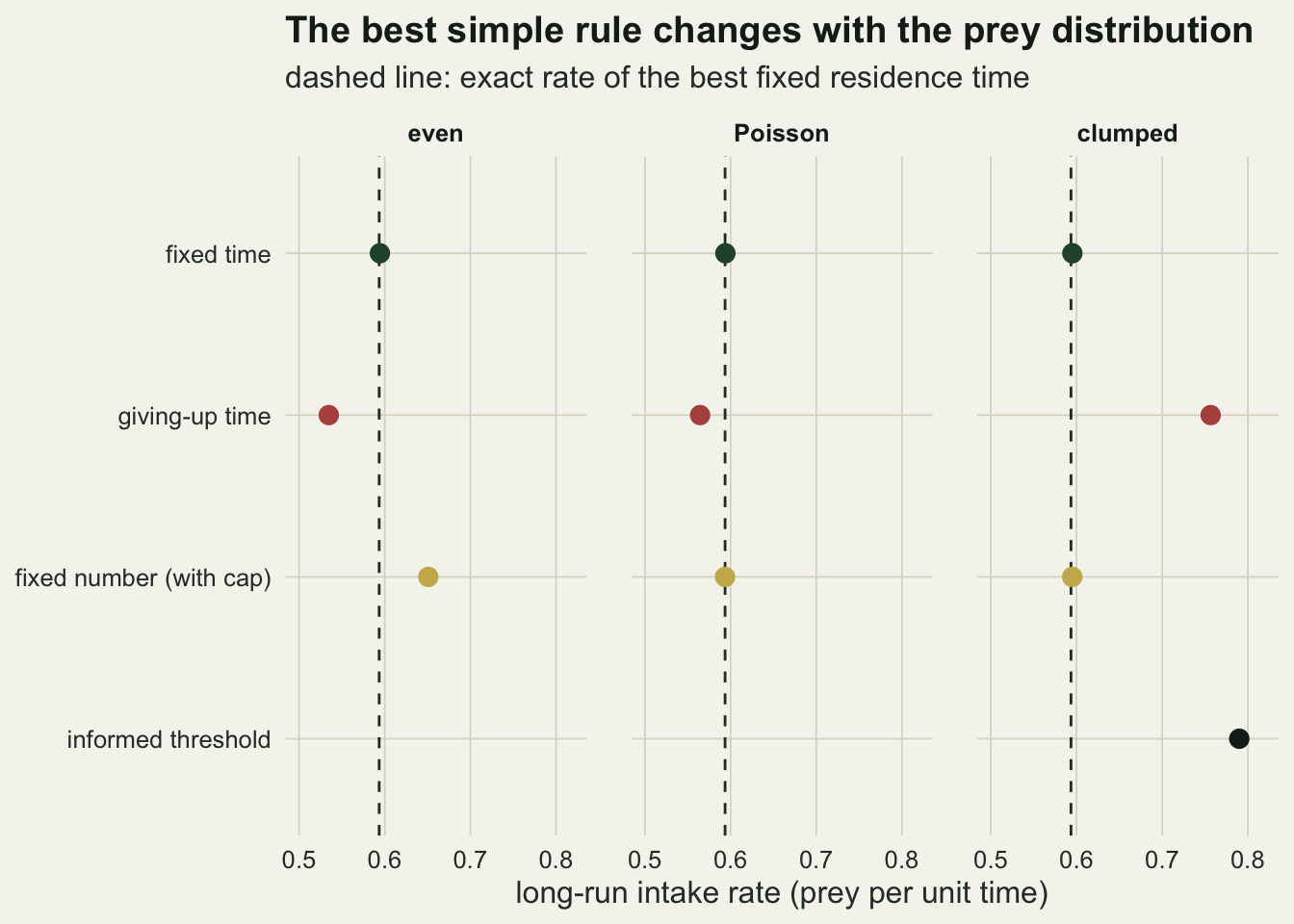
How much clumping before the giving-up time pays
The negative binomial size parameter runs from strong clumping at small values to the Poisson distribution as it grows. Somewhere along it the giving-up-time rule stops beating the fixed-time rule. Because the fixed-time rate is exact and does not depend on the distribution, the comparison only needs the giving-up-time rule simulated, and the same patch sets can be scored at several travel times.
size_grid   <- c(1.5, 2.5, 3.5, 5, 7, 10, 15)
tau_grid    <- c(1, 2, 5)
n_rep_cross <- 5
set.seed(6607)
cross_raw <- do.call(rbind, lapply(size_grid, function(s) {
  do.call(rbind, lapply(seq_len(n_rep_cross), function(r) {
    p_a <- make_patches(rnbinom(n_patch, mu = mean_prey, size = s))
    p_b <- make_patches(rnbinom(n_patch, mu = mean_prey, size = s))
    do.call(rbind, lapply(tau_grid, function(tau) {
      g_ab <- g_vals[which.max(gut_curve(p_a, g_vals, tau))]
      g_ba <- g_vals[which.max(gut_curve(p_b, g_vals, tau))]
      gut_rate <- (gut_curve(p_b, g_ab, tau) + gut_curve(p_a, g_ba, tau)) / 2
      data.frame(size = s, rep = r, tau = tau, gut = gut_rate,
                 time = max(exact_time(tau)))
    }))
  }))
}))
cross_raw$diff <- cross_raw$gut - cross_raw$time

find_cross <- function(d_mean) {
  lx <- log(size_grid)
  i  <- which(d_mean[-length(d_mean)] > 0 & d_mean[-1] <= 0)[1]
  if (is.na(i)) return(NA_real_)
  exp(lx[i] + (lx[i + 1] - lx[i]) * d_mean[i] / (d_mean[i] - d_mean[i + 1]))
}

n_boot <- 4000
set.seed(6608)
cross_tab <- do.call(rbind, lapply(tau_grid, function(tau) {
  sub_tau   <- cross_raw[cross_raw$tau == tau, ]
  sub_tau   <- sub_tau[order(sub_tau$size, sub_tau$rep), ]
  d_mat <- matrix(sub_tau$diff, nrow = n_rep_cross)
  m_d   <- colMeans(d_mat)
  se_d  <- apply(d_mat, 2, sd) / sqrt(n_rep_cross)
  est   <- find_cross(m_d)
  boot  <- replicate(n_boot, find_cross(m_d + se_d *
             rt(length(size_grid), df = n_rep_cross - 1)))
  data.frame(tau = tau, cross = est,
             lo = unname(quantile(boot, 0.025, na.rm = TRUE)),
             hi = unname(quantile(boot, 0.975, na.rm = TRUE)),
             n_na = sum(is.na(boot)), rate_time = max(exact_time(tau)))
}))
cross_sum <- aggregate(cbind(gut, diff) ~ size + tau, cross_raw, mean)
cross_sum$se <- aggregate(diff ~ size + tau, cross_raw,
                          function(x) sd(x) / sqrt(length(x)))$diff
max_se_cross <- max(cross_sum$se)
ct <- function(tau, col) cross_tab[cross_tab$tau == tau, col]
rel_adv <- function(tau) {
  row_min <- cross_sum[cross_sum$tau == tau & cross_sum$size == min(size_grid), ]
  row_min$diff / max(exact_time(tau))
}

set.seed(7719)
bayes_size <- c(0.25, 0.5, 1, 2.5, 5, 10, 15)
bayes_tab <- do.call(rbind, lapply(bayes_size, function(s) {
  p_a  <- make_patches(rnbinom(n_patch, mu = mean_prey, size = s))
  p_b  <- make_patches(rnbinom(n_patch, mu = mean_prey, size = s))
  h_ab <- h_vals[which.max(bayes_curve(p_a, h_vals, s, tau_main))]
  g_ab <- g_vals[which.max(gut_curve(p_a, g_vals, tau_main))]
  data.frame(size = s, bayes = bayes_curve(p_b, h_ab, s, tau_main),
             gut = gut_curve(p_b, g_ab, tau_main))
}))
bayes_share <- (bayes_tab$gut - rate_star) / (bayes_tab$bayes - rate_star)
share_small <- bayes_share[bayes_tab$size == 0.25]
share_one   <- bayes_share[bayes_tab$size == 1]
bayes_top   <- bayes_tab$bayes[bayes_tab$size == 15] - rate_star
With 5 independent pairs of patch sets at each of 7 size values, the standard error of the mean difference between the two rules is at most 0.0025 prey per unit time. The crossing point was located by linear interpolation of the mean difference on the log size scale, and its interval comes from 4000 draws in which the mean difference at each size is shifted by its standard error times an independent t variate with 4 degrees of freedom (the size values use separate patch sets). The 2.5 and 97.5 percentiles of the resulting crossing points give an approximate 95 per cent interval; a percentile bootstrap over only five pairs would ignore how poorly five values estimate a standard error.
At the design travel time of 2, the giving-up-time rule stops beating the fixed-time rule at a size of 4.58, with an interval from 4.19 to 5.28. A negative binomial with a mean of 5 and that size has a variance 2.1 times its mean. For negative binomial patches under these constants, then, the giving-up time wins when the variance of prey per patch exceeds about 2.1 times the mean, and the fixed clock wins below that.
cross_two <- cross_sum[cross_sum$tau == tau_main, ]
ggplot() +
  annotate("rect", xmin = ct(2, "lo"), xmax = ct(2, "hi"), ymin = -Inf, ymax = Inf,
           fill = te_line, alpha = 0.8) +
  geom_hline(yintercept = rate_star, linetype = "dashed", colour = te_forest, linewidth = 0.7) +
  geom_line(data = cross_two, aes(size, gut), colour = te_rust, linewidth = 0.9) +
  geom_point(data = cross_two, aes(size, gut), colour = te_rust, size = 2.4) +
  geom_point(data = bayes_tab, aes(size, gut), colour = te_rust, size = 2.4, shape = 21,
             fill = te_paper, stroke = 1.1) +
  geom_point(data = bayes_tab, aes(size, bayes), colour = te_ink, size = 2.4, shape = 17) +
  annotate("text", x = 0.3, y = rate_star, label = "fixed time (exact)", vjust = -0.6,
           hjust = 0, colour = te_forest, size = 3.6) +
  annotate("text", x = 1.15, y = bayes_tab$bayes[bayes_tab$size == 1] + 0.012,
           label = "informed threshold", hjust = 0,
           colour = te_ink, size = 3.6) +
  annotate("text", x = 1.2, y = 0.66, label = "giving-up time", hjust = 0,
           colour = te_rust, size = 3.6) +
  scale_x_log10(breaks = c(0.25, 0.5, 1, 2.5, 5, 10, 15),
                labels = c("0.25", "0.5", "1", "2.5", "5", "10", "15")) +
  labs(x = "negative binomial size (smaller is more clumped)",
       y = "long-run intake rate",
       title = "The giving-up time pays only under clumping",
       subtitle = "mean of five prey per patch; travel time two") +
  theme_datasheet()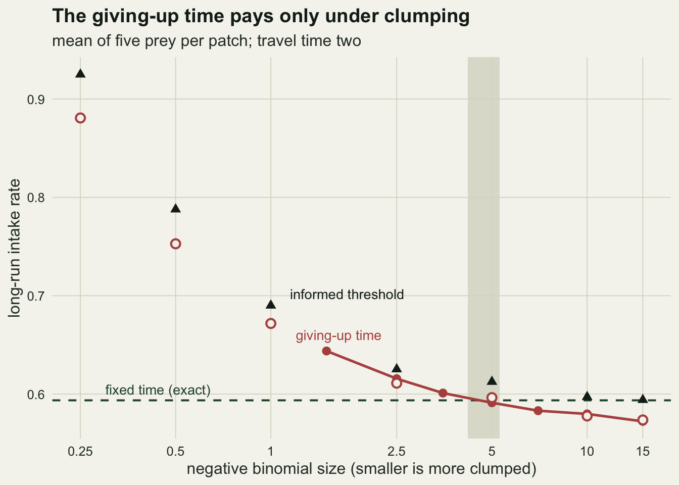
The informed threshold rule puts the giving-up-time result in scale. Measured as the share of the informed rule’s gain over the fixed-time rate that the giving-up time recovers, it gets 0.87 of it at a size of 0.25 and 0.81 at a size of 1. At a size of 15, near the Poisson end, the informed rule is only 0.0005 above the exact fixed-time rate, as the Poisson result says it should be in the limit.
cross_sum$tau_lab <- factor(sprintf("travel time %g", cross_sum$tau),
                            levels = sprintf("travel time %g", tau_grid))
cross_tab$tau_lab <- factor(sprintf("travel time %g", cross_tab$tau),
                            levels = sprintf("travel time %g", tau_grid))
tau_cols <- setNames(c(te_rust, te_forest, te_gold), levels(cross_sum$tau_lab))
ggplot(cross_sum, aes(size, diff, colour = tau_lab)) +
  geom_hline(yintercept = 0, linetype = "dashed", colour = te_body, linewidth = 0.5) +
  geom_line(linewidth = 0.9) +
  geom_point(size = 2) +
  geom_errorbar(data = cross_tab, aes(y = 0, xmin = lo, xmax = hi), inherit.aes = FALSE,
                orientation = "y", width = 0.006, colour = te_ink, linewidth = 0.6) +
  geom_point(data = cross_tab, aes(x = cross, y = 0, colour = tau_lab),
             size = 3.4, shape = 21, fill = te_paper, stroke = 1.2) +
  scale_colour_manual(values = tau_cols, name = NULL) +
  scale_x_log10(breaks = size_grid) +
  labs(x = "negative binomial size (smaller is more clumped)",
       y = "giving-up time minus fixed time (rate)",
       title = "Longer travel needs more clumping to favour the giving-up time",
       subtitle = "points: crossing points with approximate 95 per cent t-based intervals") +
  theme_datasheet() +
  theme(legend.position = "bottom")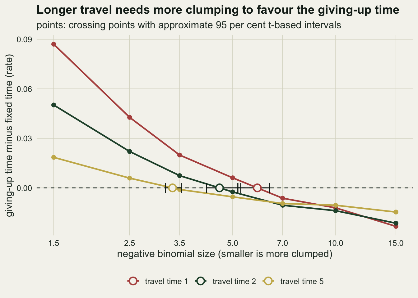
The crossing point moves with travel time. At a travel time of 1 the giving-up time wins up to a size of 5.90 (interval 5.18 to 6.41), at 2 up to 4.58, and at 5 only up to 3.34 (interval 3.18 to 3.54). The intervals for travel times 1 and 2 overlap slightly, so that step is less certain than the step from 2 to 5, where they do not. The advantage shrinks in relative terms as well as absolute ones: at the most clumped size in the grid, 1.5, the giving-up time is ahead of the clock by a fraction 0.115 of the fixed-time rate at a travel time of 1 and by 0.047 at a travel time of 5. The simulation does not isolate why, and the post does not claim a mechanism. A statement of the form “a giving-up time is best for clumped prey” needs a travel time attached before it becomes a number.
What to report
State the rule and the currency together. A residence time, a count and a giving-up time are different decision variables, and the comparison only means something when each rule’s parameter was optimised for the same long-run rate including travel. Say how the parameter was found, and if it was fitted and scored on the same simulated or observed visits, say that too.
Report the between-patch distribution of prey, not just the mean. Every rule here was run at the same mean of 5 prey per patch, and no simple rule was best for all three distributions. A variance to mean ratio, or a fitted negative binomial size, is the number that tells a reader which rule to expect.
If the argument is that animals use a giving-up time, report the travel time and the clumping together, because the crossing point moved from a size of 5.90 to 3.34 between the shortest and the longest travel time used here. Iwasa and colleagues also point to a direct empirical check: under the informed rule, residence time should rise with the number of captures on clumped prey, fall with it on even prey, and be unrelated to it on Poisson prey. A plot of captures against residence time per patch is cheap to make from any foraging record and says more than a single mean residence time.
Honest limits
Random search with exponential waiting times shapes the giving-up-time result. Every waiting time is memoryless, so a long gap is honest evidence of a poor patch, and that is the information the rule reads. A forager that searches systematically finds prey at more regular intervals and exhausts a patch completely, and a giving-up time then behaves differently; nothing here measures that case.
The fixed-number rule needed a time cap to be defined at all, and that cap turns it into a two-parameter family that contains the fixed-time rule. Its near ties with the fixed-time rule on Poisson and clumped patches are therefore partly built in: the optimiser can always switch the count off. A pure number rule with a giving-up time as its fallback would be a different family, and might inherit some of the giving-up-time rule’s advantage on clumped patches.
The informed threshold rule is a ceiling for the simple rules only in the loose sense. It leaves when the expected capture rate right now falls below a threshold, which is the form of strategy Iwasa and colleagues describe, but a myopic threshold is not guaranteed to be the optimal stopping rule when captures can raise the estimate; McNamara (1982) treats the full problem. It is also only computed for negative binomial patches, where the closed form is available.
Handling time is zero, patches do not vary in anything but prey count, travel time is fixed, and the forager knows the between-patch distribution exactly. Each of those is a simplification the original model shares. A real forager has to learn the distribution, and a giving-up time has a form that does not need that knowledge, although here its parameter G was tuned with the distribution known, so its robustness without that knowledge is not measured; the informed rule may lose its edge when its assumed size parameter is wrong, which is not measured either.
The crossing point rests on 5 replicate pairs at 7 size values and on linear interpolation between grid points. The t-based interval reflects the replicate noise but not the interpolation error, and with five replicates its width is itself uncertain. The crossing is also for one mean prey count and one search rate; it should be read as showing how the crossing moves, not as a constant.
References
Iwasa Y, Higashi M, Yamamura N 1981 The American Naturalist 117(5):710-723 (10.1086/283754)
Charnov EL 1976 Theoretical Population Biology 9(2):129-136 (10.1016/0040-5809(76)90040-X)
McNamara J 1982 Theoretical Population Biology 21(2):269-288 (10.1016/0040-5809(82)90018-1)