---
title: "The marginal value theorem"
description: "The marginal value theorem in R: the optimal time to leave a patch, the tangent that solves it, and why a richer environment means leaving each patch sooner."
date: "2026-06-30 11:00"
categories: [ecology tutorial, R, foraging, behaviour, optimisation]
image: thumbnail.png
image-alt: "A patch gain curve with a tangent line drawn from the travel time on the negative axis, touching the curve at the optimal departure time."
---
```{r setup}
#| code-fold: true
#| code-summary: "Setup: packages, colours and plot theme"
#| results: hide
#| message: false
#| warning: false
knitr::opts_chunk$set(echo = TRUE, message = FALSE, warning = FALSE,
                      dev = "png", dpi = 120, fig.path = "figures/",
                      fig.width = 7, fig.height = 4.4)
library(ggplot2)
theme_te <- theme_minimal(base_size = 12) +
  theme(panel.background = element_rect(fill = "#f5f4ee", colour = NA),
        plot.background  = element_rect(fill = "#f5f4ee", colour = NA),
        panel.grid.minor = element_blank(),
        plot.title = element_text(face = "bold", size = 12))
theme_set(theme_te)
col_gain <- "#3a6b52"; col_tan <- "#b5651d"; col_ref <- "#555555"

Gmax <- 30; k <- 0.18
g  <- function(t) Gmax * (1 - exp(-k * t))
gp <- function(t) Gmax * k * exp(-k * t)
tstar <- function(travel) uniroot(function(t) gp(t) - g(t)/(t + travel), c(1e-6, 200))$root

trav <- c(2, 6, 12)
ts   <- sapply(trav, tstar)
rate <- g(ts) / (ts + trav)
marg <- gp(ts)                      # marginal gain at departure equals the long-run rate
tab  <- data.frame(travel = trav, t_star = ts, intake = g(ts), rate = rate, marginal = marg)
```
A hummingbird works a patch of flowers, or a bee a clump of clover, and the nectar it collects piles up fast at first and then slows as the patch empties. At some point it should give up this patch and fly to the next, spending time in transit that yields nothing. When should it leave? The marginal value theorem answers this, and its answer is one of the cleaner results in behavioural ecology (Charnov 1976 Theoretical Population Biology 9(2):129-136).
## The problem
Two ingredients. Inside a patch, cumulative intake follows a gain curve `g(t)` that rises with diminishing returns. Between patches there is a travel time that returns nothing. A forager that keeps doing this collects, over the long run, a rate of
$$R(t) = \frac{g(t)}{t + \text{travel}},$$
intake per patch divided by the total time per patch, foraging plus travel. The forager should pick the residence time `t` that makes this long-run rate as large as possible.
```{r gain}
Gmax <- 30; k <- 0.18
g  <- function(t) Gmax * (1 - exp(-k * t))    # patch gain curve, diminishing returns
gp <- function(t) Gmax * k * exp(-k * t)      # marginal gain (its slope)
```
## The rule, and its picture
Maximising the long-run rate gives a strikingly simple condition: leave the patch when the *marginal* intake rate, the slope of the gain curve at that instant, has fallen to the *long-run* rate you could get by leaving now and starting fresh elsewhere.
$$g'(t^{*}) = \frac{g(t^{*})}{t^{*} + \text{travel}}.$$
Solve it with `uniroot`.
```{r solve}
tstar <- function(travel) uniroot(function(t) gp(t) - g(t)/(t + travel), c(1e-6, 200))$root
sapply(c(2, 6, 12), tstar)          # optimal residence at three travel times
```
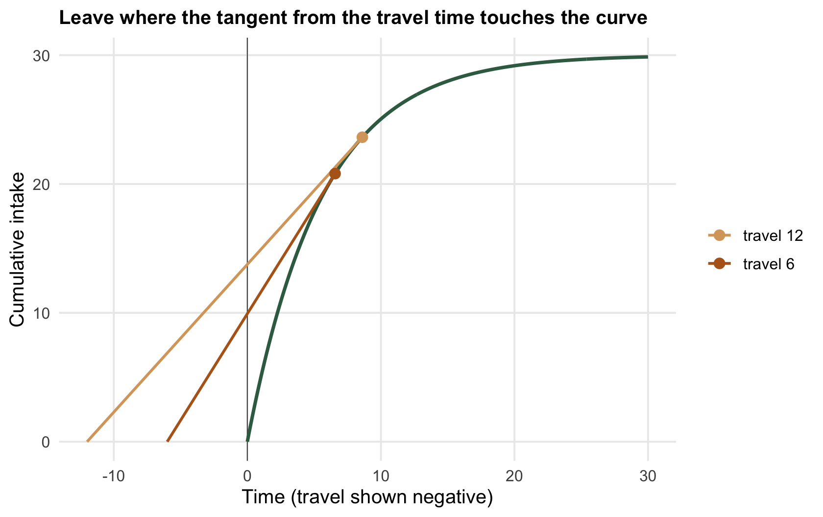
Geometrically this is a tangent. Draw the gain curve, mark the travel time as a point on the negative time axis at `(-travel, 0)`, and draw the steepest line from that point that touches the curve. It touches at the optimal departure time, and its slope is the best achievable long-run rate. The construction makes the answer visible.
```{r fig-tangent}
#| fig-cap: "The marginal value theorem as a tangent. From the travel time on the negative axis, the line touching the gain curve marks the optimal departure. A longer travel time (lighter) shifts the tangent point to the right: stay longer."
#| fig-alt: "A patch gain curve with two tangent lines drawn from two travel times on the negative axis; the tangent from the longer travel time touches the curve further to the right."
tt <- seq(0, 30, 0.1)
gc <- data.frame(t = tt, g = g(tt))
tan_df <- do.call(rbind, lapply(c(6, 12), function(tr) {
  ts <- tstar(tr); data.frame(x = c(-tr, ts), y = c(0, g(ts)), travel = paste("travel", tr))
}))
pt_df <- data.frame(t = sapply(c(6, 12), tstar), g = g(sapply(c(6, 12), tstar)),
                    travel = paste("travel", c(6, 12)))
ggplot() +
  geom_vline(xintercept = 0, colour = col_ref, linewidth = 0.3) +
  geom_line(data = gc, aes(t, g), colour = col_gain, linewidth = 1) +
  geom_line(data = tan_df, aes(x, y, group = travel, colour = travel), linewidth = 0.8) +
  geom_point(data = pt_df, aes(t, g, colour = travel), size = 2.6) +
  scale_colour_manual(values = c("travel 6" = col_tan, "travel 12" = "#d8a56b")) +
  labs(x = "Time (travel shown negative)", y = "Cumulative intake", colour = NULL,
       title = "Leave where the tangent from the travel time touches the curve")
```
## The counterintuitive part
Read the table of solutions and one number moves the wrong way for most people's intuition.
```{r table}
data.frame(travel = c(2, 6, 12),
           residence = round(sapply(c(2, 6, 12), tstar), 2),
           long_run_rate = round(sapply(c(2, 6, 12), function(tr) { ts <- tstar(tr); g(ts)/(ts+tr) }), 3))
```
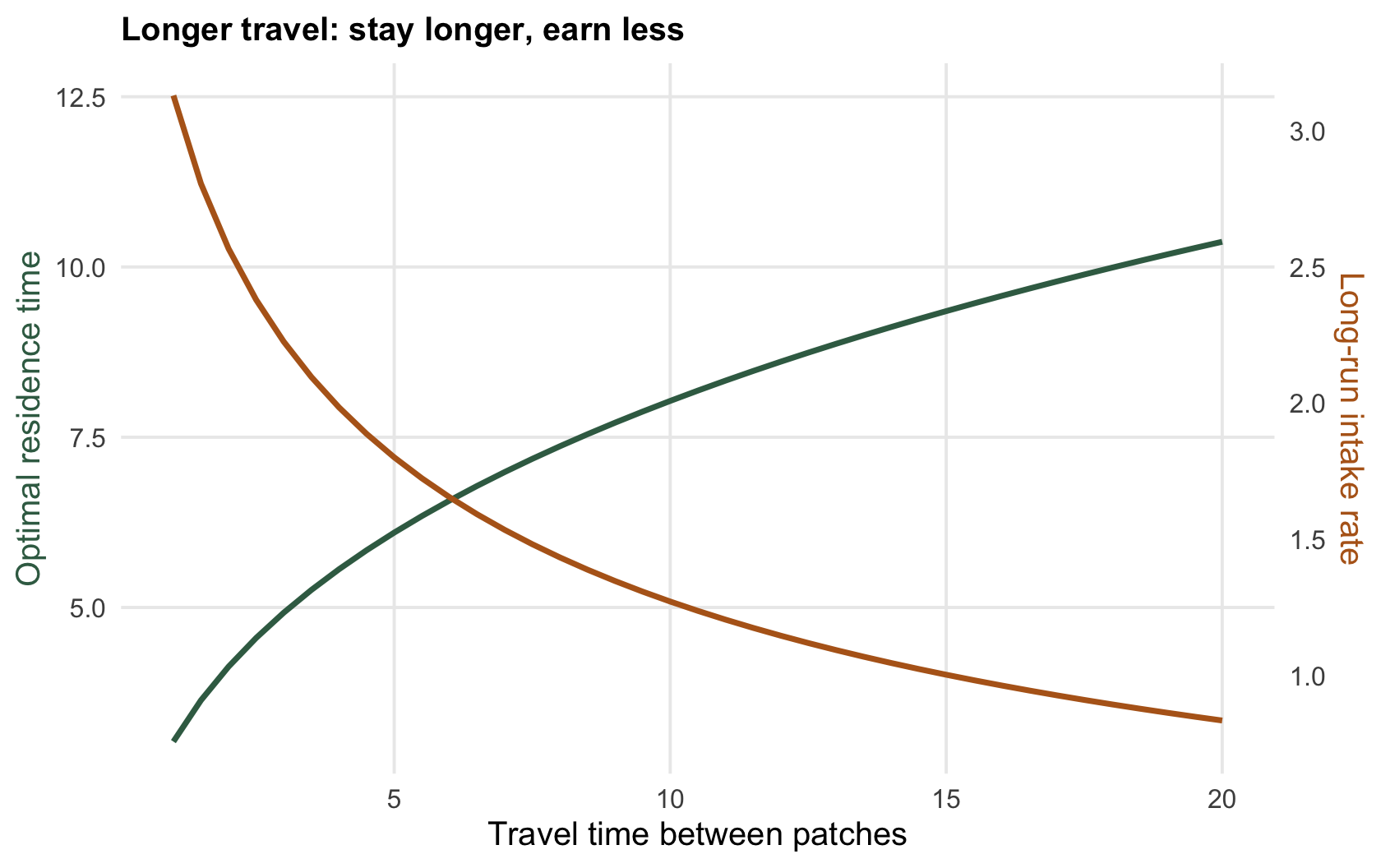
When travel time is short, `r sprintf("%.0f", trav[1])`, the forager should leave each patch after only `r sprintf("%.1f", ts[1])` time units; when travel is long, `r sprintf("%.0f", trav[3])`, it should stay `r sprintf("%.1f", ts[3])`. A richer environment, one where patches are close together and travel is cheap, means *leaving each patch sooner*, not later. It feels backwards: surely a good environment lets you relax? But the logic is opportunity cost. When the next patch is a short hop away, the rate you forgo by lingering in a depleting patch is high, so you should cut and run early. When the next patch is far, there is little to rush to, so you stay and squeeze more from the one you are in.
There is a second way to say the same thing. At the optimal departure the marginal capture rate equals the habitat-wide average rate: here the forager leaves when the patch has dropped to a marginal rate of `r sprintf("%.3f", marg[2])` at travel `r sprintf("%.0f", trav[2])`, exactly the long-run rate `r sprintf("%.3f", rate[2])` it earns overall. Quit a patch the moment it falls to the average of the whole habitat.
```{r fig-travel}
#| fig-cap: "Optimal residence time (green) rises with travel time while the long-run intake rate (ochre) falls. Cheaper travel means shorter patch visits and a higher overall rate."
#| fig-alt: "Two curves against travel time: optimal residence time rising, and long-run intake rate falling."
tr <- seq(1, 20, 0.5)
dd <- data.frame(travel = tr,
                 residence = sapply(tr, tstar),
                 rate = sapply(tr, function(x) { ts <- tstar(x); g(ts)/(ts+x) }))
ggplot(dd, aes(travel)) +
  geom_line(aes(y = residence), colour = col_gain, linewidth = 1) +
  geom_line(aes(y = rate * 4), colour = col_tan, linewidth = 1) +
  scale_y_continuous(name = "Optimal residence time",
                     sec.axis = sec_axis(~ . / 4, name = "Long-run intake rate")) +
  labs(x = "Travel time between patches",
       title = "Longer travel: stay longer, earn less") +
  theme(axis.title.y.left = element_text(colour = col_gain),
        axis.title.y.right = element_text(colour = col_tan))
```
## What the theorem assumes
The marginal value theorem is a prediction about an idealised forager: one that knows the shape of the gain curve, knows the average quality of its habitat, and is paid purely in intake rate. Real animals do not solve calculus at the flower. They use rules of thumb, leave when the capture rate drops below a threshold, or after a fixed unrewarded interval, and these approximate the theorem well without needing its knowledge. Whether an animal maximises its gross rate of intake, its net rate after metabolism or its safety is a separate question the [checking post](../checking-a-foraging-analysis/) takes up. The theorem is a benchmark for how a rate-maximiser should behave, and departures from it are how you find out what the animal is really doing. The next post keeps the forager still and asks a different question: of the prey it meets, which ones are worth eating?
## References
- Charnov EL 1976. Theoretical Population Biology 9(2):129-136 (10.1016/0040-5809(76)90040-X).
- MacArthur RH, Pianka ER 1966. The American Naturalist 100(916):603-609 (10.1086/282454).
- Pyke GH 1984. Annual Review of Ecology and Systematics 15(1):523-575 (10.1146/annurev.es.15.110184.002515).
## Related tutorials
- [Functional responses in R](../functional-responses-holling/)
- [Diet choice and the zero-one rule](../diet-choice-and-the-zero-one-rule/)
- [Checking a foraging analysis](../checking-a-foraging-analysis/)
- [Patch-leaving rules and prey clumping](../patch-leaving-rules-and-prey-clumping/)