Measure natural selection on correlated traits in R: the differential captures total selection, the gradient isolates direct selection by multiple regression.
Author
Tidy Ecology
Published
2026-07-05
Modified
2026-10-15
Corrected 15 October 2026: the post said that multiple regression inverts the phenotypic covariance matrix under the hood; it now says that the regression computes the same quantity, with lm() using a QR decomposition of the data instead.
A field biologist who measures survival or reproduction against a trait faces a quiet problem: traits travel in groups. Body size correlates with growth rate, which correlates with timing, which correlates with condition. If bigger animals leave more offspring, is size itself the target, or is size just a passenger on some other trait that selection actually favours? The answer separates two quantities that beginners often blur together: the selection differential and the selection gradient.
This post builds both from a simulated population, all in base R, and shows the matrix identity that connects them. It is the measurement half of evolutionary quantitative genetics; the breeder’s equation is the prediction half.
Total selection: the differential
The selection differential S for a trait is the covariance between the trait and relative fitness (absolute fitness divided by its mean). Equivalently, it is the change in the trait mean within a generation, before reproduction copies it forward. It counts all the selection a trait experiences, direct plus whatever it inherits through correlations with other selected traits.
Here is a population of 3000 individuals with two standardised traits, z1 and z2, correlated at 0.6. Fitness, the number of offspring, depends on z2 alone. Trait z1 has no causal effect on fitness whatsoever.
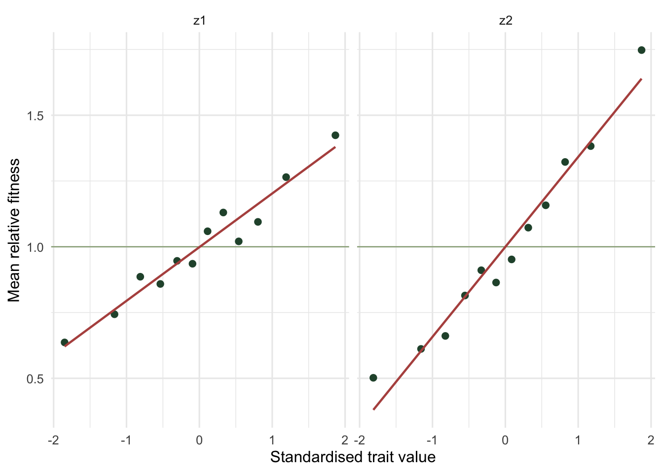
Trait z2 has a differential of 0.352, as expected. But z1 also shows a positive differential, 0.211, even though it does nothing. The ratio of the two differentials, 0.599, sits at the trait correlation of 0.6 up to sampling noise, because all z1 inherits is the correlation times the differential on z2. That is the signature of indirect selection: z1 looks selected only because it rides along with z2. A differential, on its own, cannot tell a target apart from a passenger.
Direct selection: the gradient
The selection gradient beta fixes this. It is the vector of partial regression coefficients from regressing relative fitness on all the traits at once. Because multiple regression holds the other traits constant, each gradient measures the selection acting directly on its trait, with indirect paths removed.
m <-lm(w ~ z1 + z2)beta <-coef(m)[c("z1", "z2")]round(summary(m)$coefficients, 3)
The gradient for z2 is 0.350, matching its differential because z2 is the real target. The gradient for z1 is 0.001 with a p-value of 0.954: once z2 is in the model, z1 explains nothing. The regression has stripped away the borrowed selection and left the truth. This is the core move of Lande and Arnold (1983): the differential describes what happened to each trait, the gradient describes why.
The identity that links them
The two quantities are not independent measurements; they are related through the phenotypic covariance matrix P. Collect the differentials into a vector S and the gradients into beta, and
Multiple regression computes this same quantity (lm() gets there through a QR decomposition of the data rather than by inverting P), so the two routes agree to machine precision.
Reading the identity backwards is just as useful: S = P beta. The differential a trait experiences is its own direct gradient plus the gradients of every other trait, weighted by how strongly it covaries with them. When traits are uncorrelated, P is diagonal and each differential is just its own gradient scaled by that trait’s variance; nothing is borrowed. Standardise those uncorrelated traits to unit variance and the two coincide exactly. Correlations, as here, are what pull them apart.
Figure 1: Relative fitness rises with both traits (binned means), so both have positive selection differentials. The rise in z1 is entirely borrowed through its correlation with z2.
An honest limit
Both quantities are phenotypic and descriptive. The gradient isolates direct selection only among the traits you actually measured. If some unmeasured trait causes fitness and correlates with z1, it re-enters the gradient as if z1 were the cause, exactly the omitted-variable problem of any regression (see collinearity and VIF for the standard-error side of this). A selection gradient is the best linear description of who dies and who breeds; turning it into a statement about adaptation still needs the trait to be heritable and the analysis to be honest about what was left out. That heritability step is where the breeder’s equation comes in, and the checking post walks through the assumptions that can quietly break a gradient analysis.
R version 4.5.3 (2026-03-11), aarch64-apple-darwin20
Packages: ggplot2 4.0.3
Newsletter
Get updates by email
An occasional email when tutorials are added or substantially corrected. No spam; unsubscribe anytime.
By subscribing you agree to receive these emails and confirm your address once. See the privacy policy.
ESC
Type to search the tutorials
Source Code
---title: "Selection differentials and gradients in R"description: "Measure natural selection on correlated traits in R: the differential captures total selection, the gradient isolates direct selection by multiple regression."date: "2026-07-05 14:00"date-modified: "2026-10-15"categories: [evolutionary ecology, quantitative genetics, natural selection, R, ecology tutorial]image: thumbnail.pngimage-alt: "A single panel of grouped bars comparing selection differentials and gradients for a pair of correlated traits. On the first trait the differential is about 0.21 and the gradient near zero; on the second both sit at about 0.35."---*Corrected 15 October 2026: the post said that multiple regression inverts the phenotypic covariance matrix under the hood; it now says that the regression computes the same quantity, with `lm()` using a QR decomposition of the data instead.*A field biologist who measures survival or reproduction against a trait faces a quiet problem: traits travel in groups. Body size correlates with growth rate, which correlates with timing, which correlates with condition. If bigger animals leave more offspring, is size itself the target, or is size just a passenger on some other trait that selection actually favours? The answer separates two quantities that beginners often blur together: the selection differential and the selection gradient.This post builds both from a simulated population, all in base R, and shows the matrix identity that connects them. It is the measurement half of evolutionary quantitative genetics; the [breeder's equation](../the-breeders-equation/) is the prediction half.## Total selection: the differentialThe selection differential `S` for a trait is the covariance between the trait and *relative* fitness (absolute fitness divided by its mean). Equivalently, it is the change in the trait mean within a generation, before reproduction copies it forward. It counts all the selection a trait experiences, direct plus whatever it inherits through correlations with other selected traits.Here is a population of 3000 individuals with two standardised traits, `z1` and `z2`, correlated at 0.6. Fitness, the number of offspring, depends on `z2` alone. Trait `z1` has no causal effect on fitness whatsoever.```{r}#| label: simulateset.seed(431)n <-3000rho <-0.6z2 <-rnorm(n)z1 <- rho * z2 +sqrt(1- rho^2) *rnorm(n) # cor(z1, z2) = 0.6, both ~ N(0, 1)W <-rpois(n, exp(0.30+0.35* z2)) # offspring: driven by z2 onlyw <- W /mean(W) # relative fitnessS1 <-cov(z1, w)S2 <-cov(z2, w)cat(sprintf("S1 = %.3f S2 = %.3f S1/S2 = %.3f\n", S1, S2, S1 / S2))```Trait `z2` has a differential of 0.352, as expected. But `z1` also shows a positive differential, 0.211, even though it does nothing. The ratio of the two differentials, 0.599, sits at the trait correlation of 0.6 up to sampling noise, because all `z1` inherits is the correlation times the differential on `z2`. That is the signature of indirect selection: `z1` looks selected only because it rides along with `z2`. A differential, on its own, cannot tell a target apart from a passenger.## Direct selection: the gradientThe selection gradient `beta` fixes this. It is the vector of partial regression coefficients from regressing relative fitness on all the traits at once. Because multiple regression holds the other traits constant, each gradient measures the selection acting *directly* on its trait, with indirect paths removed.```{r}#| label: gradientsm <-lm(w ~ z1 + z2)beta <-coef(m)[c("z1", "z2")]round(summary(m)$coefficients, 3)```The gradient for `z2` is 0.350, matching its differential because `z2` is the real target. The gradient for `z1` is 0.001 with a p-value of 0.954: once `z2` is in the model, `z1` explains nothing. The regression has stripped away the borrowed selection and left the truth. This is the core move of Lande and Arnold (1983): the differential describes what happened to each trait, the gradient describes why.## The identity that links themThe two quantities are not independent measurements; they are related through the phenotypic covariance matrix `P`. Collect the differentials into a vector `S` and the gradients into `beta`, and$$\boldsymbol{\beta} = \mathbf{P}^{-1}\mathbf{S}.$$Multiple regression computes this same quantity (`lm()` gets there through a QR decomposition of the data rather than by inverting `P`), so the two routes agree to machine precision.```{r}#| label: identityP <-cov(cbind(z1, z2))S <-c(S1, S2)beta_mat <-solve(P) %*% Scat(sprintf("beta (regression): %.3f %.3f\n", beta[1], beta[2]))cat(sprintf("beta (P^-1 S) : %.3f %.3f\n", beta_mat[1], beta_mat[2]))cat(sprintf("largest difference: %.1e\n", max(abs(beta_mat - beta))))```Reading the identity backwards is just as useful: `S = P beta`. The differential a trait experiences is its own direct gradient plus the gradients of every other trait, weighted by how strongly it covaries with them. When traits are uncorrelated, `P` is diagonal and each differential is just its own gradient scaled by that trait's variance; nothing is borrowed. Standardise those uncorrelated traits to unit variance and the two coincide exactly. Correlations, as here, are what pull them apart.```{r}#| label: fig-marginal#| fig-cap: "Relative fitness rises with both traits (binned means), so both have positive selection differentials. The rise in z1 is entirely borrowed through its correlation with z2."#| fig-alt: "Two panels of binned mean relative fitness against trait z1 and trait z2; both slope upward, z2 more steeply."library(ggplot2)te_canvas <-theme(plot.background =element_rect(fill ="#f5f4ee", colour =NA),panel.background =element_rect(fill ="#f5f4ee", colour =NA))bin_mean <-function(x, w, k =12) { br <-quantile(x, seq(0, 1, length.out = k +1)) gr <-cut(x, br, include.lowest =TRUE)data.frame(x =tapply(x, gr, mean), w =tapply(w, gr, mean))}d <-rbind(data.frame(trait ="z1", bin_mean(z1, w)),data.frame(trait ="z2", bin_mean(z2, w)))ggplot(d, aes(x, w)) +geom_hline(yintercept =1, colour ="#93a87f", linewidth =0.4) +geom_point(colour ="#275139", size =2) +geom_smooth(method ="lm", formula = y ~ x, se =FALSE, colour ="#b5534e", linewidth =0.8) +facet_wrap(~ trait) +labs(x ="Standardised trait value", y ="Mean relative fitness") +theme_minimal(base_size =12) + te_canvas```## An honest limitBoth quantities are phenotypic and descriptive. The gradient isolates direct selection only among the traits you actually measured. If some unmeasured trait causes fitness and correlates with `z1`, it re-enters the gradient as if `z1` were the cause, exactly the omitted-variable problem of any regression (see [collinearity and VIF](../collinearity-and-vif/) for the standard-error side of this). A selection gradient is the best linear description of who dies and who breeds; turning it into a statement about adaptation still needs the trait to be heritable and the analysis to be honest about what was left out. That heritability step is where the [breeder's equation](../the-breeders-equation/) comes in, and the [checking post](../checking-a-selection-analysis/) walks through the assumptions that can quietly break a gradient analysis.## ReferencesLande R, Arnold SJ 1983. Evolution 37(6):1210-1226 (10.1111/j.1558-5646.1983.tb00236.x)Mitchell-Olds T, Shaw RG 1987. Evolution 41(6):1149-1161 (10.1111/j.1558-5646.1987.tb02457.x)Falconer DS, Mackay TFC 1996. Introduction to Quantitative Genetics, 4th ed. Longman. ISBN 978-0582243026## Related tutorials- [Bateman gradients from genetic parentage](../bateman-gradients-from-parentage/)- [The multivariate breeder's equation](../the-multivariate-breeders-equation/)- [Checking a selection analysis](../checking-a-selection-analysis/)- [Nonlinear selection gradients in R](../nonlinear-selection-gradients/)