The multivariate breeder’s equation

Predict multi-trait evolution in R with the Lande equation delta z = G beta: correlated responses, genetic constraints, and the line of least resistance.

Traits do not evolve one at a time. Selection on beak depth drags beak width along; selection for early flowering pulls plant height with it. The single-trait breeder’s equation cannot see this, because the inheritance of one trait leaks into another through shared genes. The multivariate version, due to Lande (1979), keeps the bookkeeping straight with a matrix:

\[ \Delta\bar{\mathbf{z}} = \mathbf{G}\boldsymbol{\beta}. \]

Here beta is the vector of selection gradients, one per trait, and G is the additive genetic variance-covariance matrix: its diagonal holds the additive variances (the raw material for each trait) and its off-diagonal holds the genetic covariances (the shared genetic basis). The response delta z-bar is what actually evolves. Everything interesting comes from G not being diagonal.

The G matrix and the line of least resistance

Take two traits with equal additive variances and a positive genetic covariance of 0.7.

set.seed(433)
G <- matrix(c(1, 0.7, 0.7, 1), 2)
ang <- function(u, v) acos(sum(u * v) / sqrt(sum(u^2) * sum(v^2))) * 180 / pi

e <- eigen(G)
cat(sprintf("eigenvalues: %.2f (gmax), %.2f (gmin)\n", e$values[1], e$values[2]))

eigenvalues: 1.70 (gmax), 0.30 (gmin)

cat(sprintf("gmax points along (%.2f, %.2f), a 45 degree diagonal\n",
            e$vectors[1, 1], e$vectors[2, 1]))

gmax points along (0.71, 0.71), a 45 degree diagonal

The leading eigenvector of G, called gmax, is the direction in trait space with the most additive genetic variance: 1.70 units along the diagonal versus only 0.30 across it. Schluter (1996) named this the genetic line of least resistance, because a population evolves fastest along it and drags its feet in any other direction. G is a covariance matrix, so this is the same eigen-decomposition that drives principal component analysis; gmax is simply the first principal component of the breeding values.

A correlated response

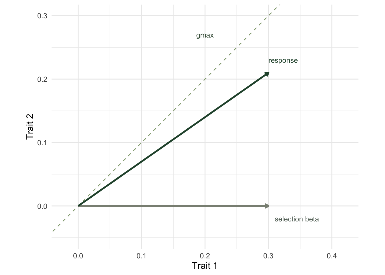
Now select on the first trait only, with a gradient of 0.3, and leave the second trait alone.

betaA <- c(0.3, 0)
dzA   <- G %*% betaA
cat(sprintf("response = (%.3f, %.3f)\n", dzA[1], dzA[2]))

response = (0.300, 0.210)

cat(sprintf("trait 2 evolves %.3f with zero direct selection; response deflected %.0f deg from beta\n",
            dzA[2], ang(dzA, betaA)))

trait 2 evolves 0.210 with zero direct selection; response deflected 35 deg from beta

cat(sprintf("response sits only %.0f deg off gmax\n", ang(dzA, e$vectors[, 1])))

response sits only 10 deg off gmax

Trait 2 moves by 0.210 even though selection never touched it. This is a correlated response: the genes that raise trait 1 also raise trait 2, so trait 2 comes along for free. The response is deflected 35 degrees away from the direction selection pushed, and it lands only 10 degrees off gmax. Selection sets the target, but G steers the outcome toward the line of least resistance.

A genetic constraint

The steering can also be a brake. Suppose selection is antagonistic: it favours a larger trait 1 and a smaller trait 2, a gradient of (0.3, -0.3). That direction runs straight across the grain of G.

betaB     <- c(0.3, -0.3)
dzB       <- G %*% betaB
dzB_indep <- diag(diag(G)) %*% betaB          # response if traits shared no genes
cat(sprintf("response magnitude with genetic correlation: %.3f\n", sqrt(sum(dzB^2))))

response magnitude with genetic correlation: 0.127

cat(sprintf("response magnitude if traits were independent: %.3f\n", sqrt(sum(dzB_indep^2))))

response magnitude if traits were independent: 0.424

cat(sprintf("the genetic correlation shrinks the response by %.0f%%\n",
            100 * (1 - sqrt(sum(dzB^2)) / sqrt(sum(dzB_indep^2)))))

the genetic correlation shrinks the response by 70%

The same selection that would produce a response of magnitude 0.424 on genetically independent traits manages only 0.127 here, a 70% reduction. The population “wants” to pull the traits apart, but the shared genes resist. This is a genetic constraint: abundant additive variance in each trait separately, yet almost none in the combination selection is trying to build. Walsh and Blows (2009) argue this near-empty direction, not any shortage of variation, is what most often limits multivariate adaptation.

Confirming it by simulation

The matrix identity is not an approximation; it falls out of the definitions. Draw breeding values from G, add environmental variation to make phenotypes, impose a linear fitness function, and the realised response matches G times the estimated gradient. It also matches the covariance between breeding value and relative fitness, the multivariate Robertson-Price identity.

n  <- 20000
E  <- matrix(c(1, 0.2, 0.2, 1), 2)                 # environmental covariance
a  <- t(t(chol(G)) %*% matrix(rnorm(2 * n), 2))    # breeding values ~ MVN(0, G)
z  <- a + t(t(chol(E)) %*% matrix(rnorm(2 * n), 2))
P  <- cov(z)
w  <- 1 + as.numeric(z %*% betaA); w[w < 0] <- 0; w <- w / mean(w)
S        <- c(cov(z[, 1], w), cov(z[, 2], w))
dz_pred  <- G %*% solve(P) %*% S                   # G P^-1 S
dz_real  <- c(cov(a[, 1], w), cov(a[, 2], w))      # cov(breeding value, fitness)
cat(sprintf("predicted G P^-1 S : (%.3f, %.3f)\n", dz_pred[1], dz_pred[2]))

predicted G P^-1 S : (0.298, 0.209)

cat(sprintf("realised cov(a, w) : (%.3f, %.3f)\n", dz_real[1], dz_real[2]))

realised cov(a, w) : (0.293, 0.201)

The prediction (0.298, 0.209) and the realised response (0.293, 0.201) agree within sampling error, and both recover the correlated response of the pure matrix calculation.

library(ggplot2)
gm <- e$vectors[, 1]
ggplot() +
  geom_abline(slope = gm[2] / gm[1], intercept = 0, linetype = "dashed", colour = "#93a87f") +
  geom_segment(aes(x = 0, y = 0, xend = betaA[1], yend = betaA[2]),
               colour = "#8a8f83", linewidth = 1.1,
               arrow = arrow(length = unit(0.18, "cm"))) +
  geom_segment(aes(x = 0, y = 0, xend = dzA[1], yend = dzA[2]),
               colour = "#275139", linewidth = 1.1,
               arrow = arrow(length = unit(0.18, "cm"))) +
  annotate("text", x = 0.31, y = -0.02, label = "selection beta", colour = "#5d6b61", size = 3.3, hjust = 0) +
  annotate("text", x = 0.30, y = 0.23, label = "response", colour = "#275139", size = 3.3, hjust = 0) +
  annotate("text", x = 0.20, y = 0.27, label = "gmax", colour = "#46604a", size = 3.3) +
  coord_equal(xlim = c(-0.02, 0.42), ylim = c(-0.05, 0.3)) +
  labs(x = "Trait 1", y = "Trait 2") +
  theme_minimal(base_size = 12)

Figure 1: Selection on trait 1 alone (grey) produces a response (green) deflected toward gmax, the genetic line of least resistance (dashed). Trait 2 evolves through the genetic covariance.

An honest limit

The Lande equation is exact given G and beta, but G is the hard part. Estimating a genetic covariance matrix needs a pedigree or known relatedness and large samples, and the off-diagonal elements are the least precise part of it. Worse, G is not fixed: it shifts with allele frequencies, environment, and the very selection acting on it, so a G measured today only forecasts the next generation or two. The response also depends on directions in trait space where genetic variance can be almost absent, and those near-empty directions are exactly where the estimates are noisiest. Checking a selection analysis takes up how much of this uncertainty a real study can actually carry.

Related tutorials

• Selection differentials and gradients
• The breeder’s equation
• Checking a selection analysis
• PCA of environmental data

References

Lande R 1979. Evolution 33(1):402-416 (10.1111/j.1558-5646.1979.tb04694.x)

Lande R, Arnold SJ 1983. Evolution 37(6):1210-1226 (10.1111/j.1558-5646.1983.tb00236.x)

Schluter D 1996. Evolution 50(5):1766-1774 (10.1111/j.1558-5646.1996.tb03563.x)

Walsh B, Blows MW 2009. Annual Review of Ecology, Evolution, and Systematics 40:41-59 (10.1146/annurev.ecolsys.110308.120232)