library(ggplot2)
library(patchwork)

te_paper  <- "#f5f4ee"
te_ink    <- "#16241d"
te_body   <- "#2c3a31"
te_forest <- "#275139"
te_rust   <- "#b5534e"
te_gold   <- "#c9b458"
te_line   <- "#dad9ca"

theme_datasheet <- function() {
  theme_minimal(base_size = 12) +
    theme(plot.background  = element_rect(fill = te_paper, colour = NA),
          panel.background = element_rect(fill = te_paper, colour = NA),
          panel.grid.major = element_line(colour = te_line, linewidth = 0.3),
          panel.grid.minor = element_blank(),
          text             = element_text(colour = te_body),
          plot.title       = element_text(colour = te_ink, face = "bold"),
          plot.subtitle    = element_text(colour = te_body),
          axis.text        = element_text(colour = te_body))
}

bin_means <- function(zz, ww, half = 3.3, step = 0.3, k_min = 20) {
  gid <- cut(zz, seq(-half, half, by = step))
  out <- data.frame(z = tapply(zz, gid, mean), wbar = tapply(ww, gid, mean),
                    k = tapply(ww, gid, length))
  out[!is.na(out$z) & out$k >= k_min, ]
}

w_true    <- 1.2
n_plant   <- 8000
seed_mean <- 12

set.seed(8201)
z_flower <- rnorm(n_plant)
surf_true <- exp(-z_flower^2 / (2 * w_true^2))
seeds  <- rpois(n_plant, seed_mean * surf_true)
w_rel  <- seeds / mean(seeds)

m_quad  <- lm(w_rel ~ z_flower + I(z_flower^2))
c_raw   <- unname(coef(m_quad)[3])
se_raw  <- summary(m_quad)$coefficients[3, 2]
gam_hat <- 2 * c_raw
b_hat   <- unname(coef(m_quad)[2])
p_trait <- var(z_flower)
seed_bar <- mean(seeds)
theta_true <- 0
q_scale    <- w_true^2 + p_trait
gam_expect <- (theta_true^2 - q_scale) / q_scale^2Nonlinear selection gradients in R
R
evolutionary ecology
quantitative genetics
natural selection
ecology tutorial
Quadratic selection gradients in R: the regression coefficient is half the gradient, and fitting one trait at a time turns a saddle into disruptive selection.
A field season ends with two columns. Flowering date for every plant in the plot, and the number of seeds each one set. Plants that flowered early met a late frost, plants that flowered late ran out of pollinators, and the mean of the survivors sits about where it started. Directional selection is not the quantity of interest here. What matters is how sharply fitness falls away on either side of the optimum, because that curvature is what holds the trait in place.
The curvature has a name, the quadratic selection gradient, and almost everyone estimates it by fitting lm(w ~ z + I(z^2)) and reading the second coefficient off the table. That coefficient is not the gradient. It is half of it. The factor of two is not a convention that some authors follow and others do not: it comes from the position of the term in a second-order expansion, where every squared term carries a one half in front of it.
A second failure costs more than a factor of two. A quadratic fitted to one trait at a time cannot separate curvature along that trait from selection on its product with another trait. Two correlated traits under pure correlational selection, with no curvature along either axis, still give a large quadratic coefficient for each trait taken by itself. Its sign follows the sign of the correlation times the correlational gradient, so the same saddle reads as disruptive selection on one pair of traits and as an optimum that is not there on another. The coefficient is real, its standard error is small, and neither reading is a fact about the trait.
This post measures both, and it measures how often a field study can see nonlinear selection at all. The linear half of the subject is covered elsewhere on the site: selection differentials and gradients fits lm(w ~ z1 + z2) and stops at the first-order terms, and the multivariate breeder’s equation turns those terms into a predicted response. What follows is the second-order term that neither of them fits, in base R, with ggplot2 for the figures.
The quadratic coefficient is half the gradient
Lande and Arnold (1983) write relative fitness as a second-order expansion in the traits:
\[ w = a + \sum_i \beta_i z_i + \frac{1}{2} \sum_i \sum_j \gamma_{ij} z_i z_j + \varepsilon . \]
The one half in front of the double sum is the same one half that stands in front of the second derivative in any Taylor expansion, and it is the whole problem. For a single trait the expansion contains the term 0.5 * gam * z^2, so the coefficient that lm returns for I(z^2) estimates gam / 2, and the gradient is twice what the table prints. For the cross-product of two different traits the double sum passes over the pair twice, once as ij and once as ji, so the two halves add to one and the coefficient of z1:z2 is the gradient already, with no doubling. Stinchcombe et al. (2008) is the paper that put this in front of the field: how often published quadratic gradients had not been doubled, and how often a paper gave the reader no way to tell which convention it had used.
Here is a population where the surface is known. Flowering date is standardised, fitness is seed set, and the surface is Gaussian with a known width. The sample is far larger than a real study of this kind, deliberately, so that the arithmetic rather than the sampling error is what shows.
8000 plants, a mean seed set of 9.2, and a trait scaled to a variance of 0.99. The fitted linear coefficient is -0.003, which is the correct answer for a surface with its optimum at the trait mean: there is no directional selection to find. The coefficient of I(z_flower^2) is -0.2059 with a standard error of 0.0028, so the quadratic selection gradient is -0.4117.
Two numbers that differ by a factor of two, both of which get called gamma in the literature. The one that belongs in the second-order expansion, and therefore the one that belongs in any calculation that uses gamma, is the doubled one. For this surface, this trait distribution and an optimum sitting at the trait mean, the value it should take is -0.4108, which is derived in the next section, and the estimate lands on it.
bin_dat <- bin_means(z_flower, w_rel)
z_fine  <- data.frame(z_flower = seq(-3.3, 3.3, length.out = 300))
curve_long <- data.frame(
  z = rep(z_fine$z_flower, 2),
  y = c(exp(-z_fine$z_flower^2 / (2 * w_true^2)) / mean(surf_true),
        predict(m_quad, z_fine)),
  which_curve = rep(c("Gaussian surface (truth)", "fitted quadratic"),
                    each = nrow(z_fine)))

ggplot(bin_dat, aes(z, wbar)) +
  geom_hline(yintercept = 0, colour = te_line, linewidth = 0.4) +
  geom_point(size = 2.2, colour = te_ink) +
  geom_line(data = curve_long, aes(z, y, colour = which_curve), linewidth = 0.9) +
  scale_colour_manual(values = c("fitted quadratic" = te_rust,
                                 "Gaussian surface (truth)" = te_forest),
                      name = NULL) +
  labs(x = "flowering date (standardised)", y = "relative fitness",
       title = "The quadratic is a local approximation",
       subtitle = "it tracks the surface near the mean and leaves it in the tails") +
  theme_datasheet() +
  theme(legend.position = "bottom")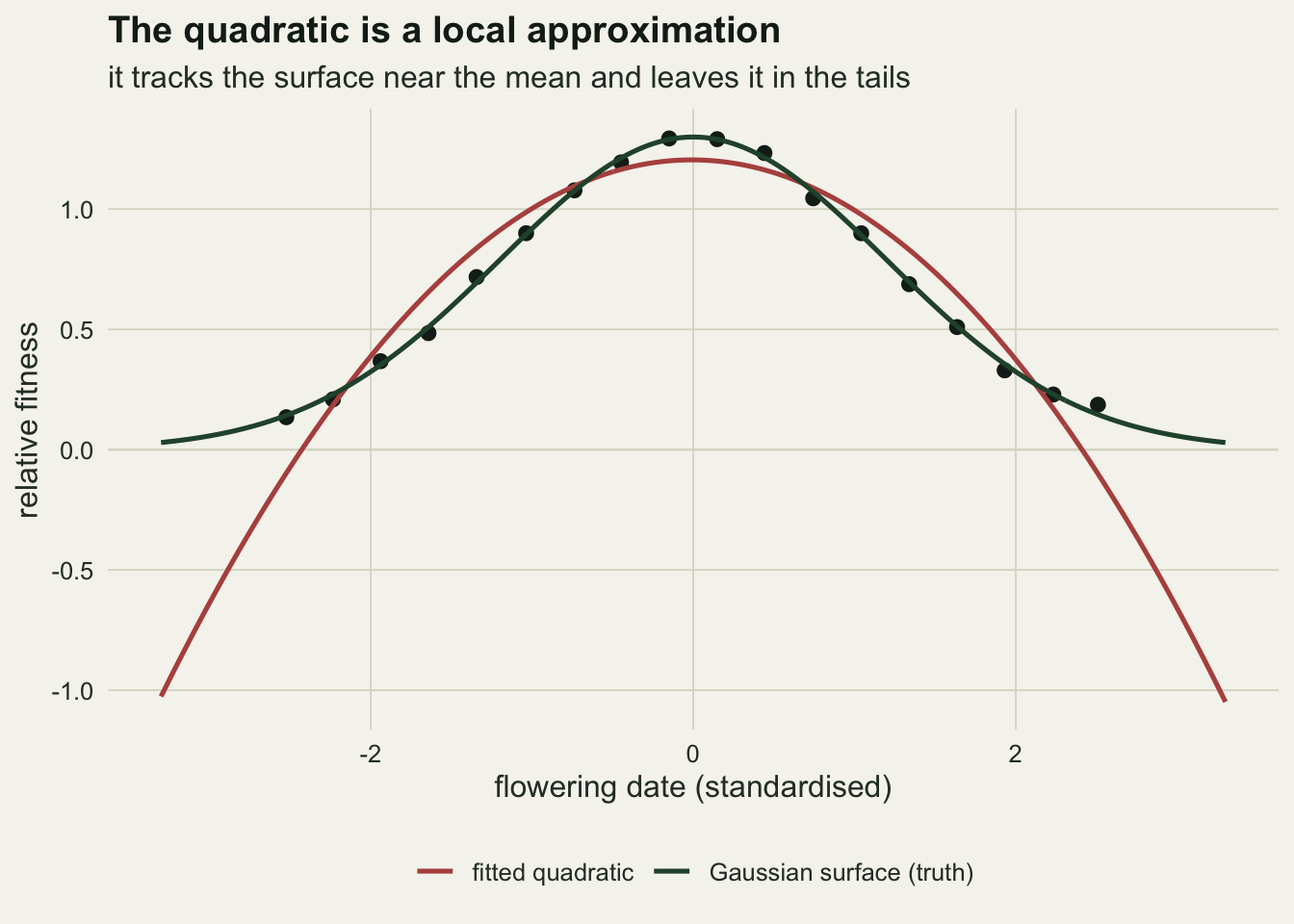
A halved gradient makes the fitness surface look much wider
The gradient is worth having because it converts into something a biologist can picture: the width of the fitness surface, the distance in trait units over which fitness falls away. For a Gaussian surface of width w with its peak at theta, and a normally distributed trait of variance P, the algebra closes exactly. The product of the trait density and the surface is itself a normal density, and working its mean and variance through the two gradients gives
\[ \beta = \frac{\theta}{w^2 + P}, \qquad \gamma = \frac{\theta^2 - (w^2 + P)}{(w^2 + P)^2} . \]
Those are one statement and not two: substitute the first into the second and what is left is gam = b^2 - 1 / (w^2 + P). Inverting that gives a width recipe, and the recipe needs both gradients,
\[ w = \sqrt{\frac{1}{\beta^2 - \gamma} - P} \; , \]
which collapses to the familiar sqrt(-1 / gam_hat - p_trait) only when the optimum sits at the trait mean, so that beta is zero. That is the case in the population above, and it is the case in almost no field population; the next section measures what the familiar form costs when it is assumed and does not hold. The term p_trait in either version is not a nuisance. A quadratic regression estimates the average curvature of the surface across the range the trait actually occupies, not the curvature at the peak, and the wider the trait is spread the flatter that average is.
w_from_grad <- sqrt(-1 / gam_hat - p_trait)
w_from_raw  <- sqrt(-1 / c_raw  - p_trait)
infl        <- w_from_raw / w_from_grad
infl_closed <- sqrt(2 + p_trait / w_true^2)
infl_floor  <- sqrt(2)
The doubled gradient returns a width of 1.198 against a true width of 1.20. The undoubled coefficient returns 1.966, a surface 64 per cent wider than the one the plants experienced, which in this population is the difference between a trait held firmly and a trait barely held at all.
That inflation factor is not an accident of these data. The two widths are both functions of the one fitted gradient, so the gradient cancels out of their ratio:
\[ \frac{\sqrt{-2/\gamma - P}}{\sqrt{-1/\gamma - P}} = \sqrt{\frac{2(w^2 + P) - P}{(w^2 + P) - P}} = \sqrt{2 + \frac{P}{w^2}} . \]
Here w is the width the doubled gradient returns, which is the true width when the optimum sits at the trait mean, as it does here. The closed form gives 1.640 and the two fitted widths give 1.641. The second term inside the square root is what strong selection contributes, and it shrinks as the surface gets wide relative to the trait. The floor is 1.414, the square root of two, and it is approached rather than reached: the trait always has some spread, so the second term is always positive. Dropping the factor of two never widens a surface by less than that, and in published data, where nonlinear selection is usually weak, the cost is not far above it.
An optimum away from the trait mean breaks the width recipe
The population above was built with its optimum at the trait mean, which is where a simulation can put it and where a field population usually is not. Move the peak to theta and the trait mean sits on a slope. The regression then sees the curvature of the surface plus a contribution from that slope, and the identity says exactly how much: gamma rises by beta squared, whatever the width. The reference strengths below are the median absolute gradients that Kingsolver et al. (2001) compiled from hundreds of published estimates.
b_lit  <- 0.16              # Kingsolver et al. (2001), median absolute gradients
g_pub  <- -0.10
n_paper <- 33               # Stinchcombe et al. (2008), papers audited
share_undoubled <- 0.78
g_dbl  <- 2 * g_pub
gam_at  <- function(ww, bb, pp) bb^2 - 1 / (pp + ww^2)
w_naive <- function(gg, pp) sqrt(-1 / gg - pp)
w_joint <- function(bb, gg, pp) sqrt(1 / (bb^2 - gg) - pp)

th_check <- c(0, 0.8, 1.6)
n_check  <- 400000
set.seed(8204)
grad_sim <- vapply(th_check, function(th) {
  z    <- rnorm(n_check, 0, sqrt(p_trait))
  surf <- exp(-(z - th)^2 / (2 * w_true^2))
  wr   <- surf / mean(surf)
  cf   <- coef(lm(wr ~ z + I(z^2)))
  c(unname(cf[2]), 2 * unname(cf[3]))
}, numeric(2))

g_pred  <- gam_at(w_true, th_check / (w_true^2 + p_trait), p_trait)
dev_max <- max(abs(grad_sim[2, ] - g_pred))
w_back  <- w_joint(grad_sim[1, ], grad_sim[2, ], p_trait)
w_flat  <- w_naive(g_pub, p_trait)
b_seq <- seq(0, 0.7, length.out = 260)
disp <- data.frame(bb = rep(b_seq, 2),
                   w0 = rep(c(w_true, w_flat), each = length(b_seq)))
disp$gam <- gam_at(disp$w0, disp$bb, p_trait)
disp$src <- factor(sprintf("true width %.1f", disp$w0))
disp_neg <- disp[disp$gam < 0, ]
disp_neg$ratio <- w_naive(disp_neg$gam, p_trait) / disp_neg$w0
err_med  <- w_naive(gam_at(w_flat, b_lit, p_trait), p_trait) / w_flat
b_str    <- 1.5 * b_lit
err_str  <- w_naive(gam_at(w_flat, b_str, p_trait), p_trait) / w_flat
b_flip_n <- 1 / sqrt(p_trait + w_true^2)
b_flip_w <- 1 / sqrt(p_trait + w_flat^2)
Three surfaces of the same width 1.2, with peaks at 0.0, 0.8 and 1.6 phenotypic standard deviations, each sampled at 400000 individuals: the fitted gradients match the closed form to within 0.0017. Feed both gradients into the joint recipe and the width comes back as 1.204, 1.198 and 1.204, against a truth of 1.20 in every case. Feed only the quadratic gradient into the familiar one and the third surface has no width at all: its gamma is positive.
That is the failure worth naming. A gradient of -0.10 read as a centred surface implies a width of 3.00 phenotypic standard deviations. Displace the optimum on a surface of that width until the directional gradient reaches the compiled median of 0.16, and the same recipe returns a width 18 per cent too large; at 0.24 it is 58 per cent too large. That is the same order as the doubling error this post exists to warn about, and it runs in the same direction, so the two compound. Past a directional gradient of 0.316 the quadratic gradient of that surface turns positive and a purely stabilising surface is reported as disruptive selection. The narrow surface holds out longer, to 0.641, which is the general rule: the flatter the surface, the less directional selection it takes to make a hill look like a valley.
disp_panel <- function(dat, yy, y0, ylab, ttl, sub, ylim = NULL) {
  ggplot(dat, aes(bb, .data[[yy]], colour = src)) +
    geom_hline(yintercept = y0, colour = te_line, linewidth = 0.4) +
    geom_vline(xintercept = b_lit, colour = te_gold, linetype = "22",
               linewidth = 0.5) +
    geom_line(linewidth = 0.9) +
    scale_colour_manual(values = c(te_forest, te_rust), name = NULL) +
    coord_cartesian(ylim = ylim) +
    labs(x = "directional gradient", y = ylab, title = ttl, subtitle = sub) +
    theme_datasheet()
}

disp_panel(disp_neg, "ratio", 1, "width recovered / true width",
           "The centred recipe inflates",
           "gold: the median published gradient", c(1, 4)) +
  disp_panel(disp, "gam", 0, "quadratic gradient", "and then changes sign",
             "above zero a hill is reported as a valley") +
  plot_layout(guides = "collect") +
  plot_annotation(theme = theme_datasheet() +
                    theme(legend.position = "bottom"))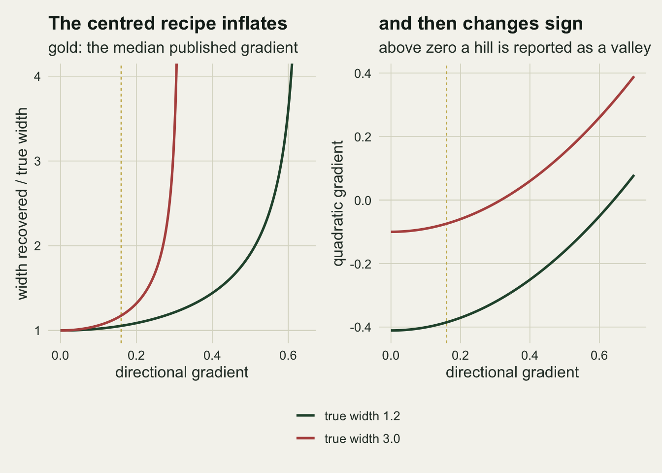
The quadratic term is the one a field study cannot detect
The gradients above came from a sample no field worker will ever have. The question here is how often a study of a given size recovers each term at the strengths the compilation reports, with fitness as a count of offspring in a population close to replacement. The generating value for the curvature is not settled, and this post is the reason. The compiled median absolute quadratic gradient is 0.10, taken here as stabilising, but Stinchcombe et al. (2008) audited 33 later papers and found that at least 78 per cent of them had not doubled. If that share is anything like representative of the studies the compilation drew on, most of the values behind the median are half-gradients and the median curvature is nearer -0.20 than -0.10. The sweep runs at both, because there is no way to tell from the compiled number which it is.
mu_fit <- 1.2
n_grid <- c(100, 200, 500, 1000, 2000)
n_rep  <- 6000
surf_floor <- 0.05
alpha_lev  <- 0.05

one_study <- function(nn, gg) {
  z <- rnorm(nn)
  surf <- 1 + b_lit * z + 0.5 * gg * (z^2 - 1)
  off  <- rpois(nn, mu_fit * pmax(surf, surf_floor))
  wr   <- off / mean(off)
  cf   <- summary(lm(wr ~ z + I(z^2)))$coefficients
  c(cf[2, 4], cf[3, 4], cf[2, 1], 2 * cf[3, 1])
}
sweep_at <- function(gg) lapply(n_grid, function(nn)
  vapply(seq_len(n_rep), function(k) one_study(nn, gg), numeric(4)))
hit_rate <- function(runs, i) vapply(runs, function(m) mean(m[i, ] < alpha_lev), 0)

set.seed(8202)
runs_pub <- sweep_at(g_pub)
set.seed(8222)
runs_dbl <- sweep_at(g_dbl)
set.seed(8212)
null_runs <- vapply(seq_len(n_rep), function(k) one_study(n_grid[1], 0), numeric(4))
det_tab <- data.frame(
  n     = n_grid,
  lin   = hit_rate(runs_pub, 1),
  quad  = hit_rate(runs_pub, 2),
  q_dbl = hit_rate(runs_dbl, 2),
  b_bar = vapply(runs_pub, function(m) mean(m[3, ]), 0),
  g_bar = vapply(runs_pub, function(m) mean(m[4, ]), 0),
  g_sd  = vapply(runs_pub, function(m) sd(m[4, ]), 0))
null_rate <- mean(null_runs[2, ] < alpha_lev)
b_worst <- max(abs(det_tab$b_bar - b_lit))
g_worst <- max(abs(det_tab$g_bar - g_pub))
size_ratio <- (b_lit / (abs(0.5 * g_pub) * sqrt(2)))^2
size_ratio_dbl <- (b_lit / (abs(0.5 * g_dbl) * sqrt(2)))^2
small <- runs_pub[[1]]
found <- small[2, ] < alpha_lev
n_found   <- sum(found)
rate_over <- det_tab$quad[1] / null_rate
se_gap    <- sqrt(det_tab$quad[1] * (1 - det_tab$quad[1]) / n_rep +
                    null_rate * (1 - null_rate) / n_rep)
gap_se    <- (det_tab$quad[1] - null_rate) / se_gap
g_found   <- mean(abs(small[4, found]))
curse     <- g_found / abs(g_pub)
wrong_way <- mean(small[4, found] > 0)
qa <- -0.5 * g_dbl
qc <- 1 - 0.5 * g_dbl - surf_floor
root_hw <- sqrt(b_lit^2 + 4 * qa * qc)
clip_frac <- pnorm((b_lit - root_hw) / (2 * qa)) +
  pnorm((b_lit + root_hw) / (2 * qa), lower.tail = FALSE)
w_dbl    <- w_naive(g_dbl, p_trait)
infl_lit <- sqrt(2 + p_trait / w_dbl^2)
Both terms are unbiased on average. Across 6000 replicates at each size the mean estimates never depart from the generating values of 0.16 and -0.10 by more than 0.0010 and 0.0014. Unbiased on average is a property of the ensemble and not of a study: the standard deviation of the estimated quadratic gradient across replicates is 0.131 at 100 individuals, larger than the gradient being estimated, and it is still 0.026 at 2000.
At 100 individuals the linear term clears the 0.05 threshold in 38 per cent of the replicates and the quadratic term in 9.0 per cent, against 4.8 per cent when the quadratic gradient is set to zero. The difference is real: 1.9 times the null rate, and 9.1 Monte Carlo standard errors from it. It is the use that fails rather than the test. Among the 540 replicates that reached significance at that size, the mean absolute gradient is 0.314, or 3.1 times the value that generated the data, and 3.3 per cent of them have the wrong sign. Conditioning on significance keeps the replicates in which noise pushed the estimate away from zero, so a quadratic gradient that is significant at a hundred individuals is not an estimate of curvature: it is an upper bound that has been selected for being large.
The picture depends on which reading of the compiled median is right. At -0.10 the quadratic term is found in 39 per cent of studies at 500 individuals and reaches 94 per cent only at 2000; at -0.20 it is already at 93 per cent by 500. The honest summary is that range, and the range is a consequence of the reporting problem: until a paper says which convention it used, its readers cannot tell which of these two power curves they are on.
The gap between the terms has an arithmetic source that no amount of care in the field will remove. The linear term multiplies z, whose standard deviation is one; the quadratic coefficient multiplies z^2, whose deviations about their mean have a standard deviation of the square root of two. With the same residual noise, the ratio of sample sizes needed for equal power is the square of the ratio of those signals, which is 5.1 at the published median and 1.3 at the doubled one. The sweep bears the first out: the linear term at 100 individuals is found in 38 per cent of studies and the quadratic term at 500 in 39 per cent.
That has a consequence for reading the literature. The published record of nonlinear selection is not a sample of what nonlinear selection is like; it is a sample of the nonlinear selection large enough to be reported, and it is thin in exactly the region where most of it lives. It also fixes the size of the doubling error in real data: read as a centred surface, a gradient of -0.10 implies a width of 3.00 phenotypic standard deviations and -0.20 implies 2.00, and the inflation from dropping the factor of two is 1.499.
lab_q <- sprintf("quadratic gradient %.2f", c(g_dbl, g_pub))
det_long <- data.frame(
  n = rep(det_tab$n, 3),
  rate = c(det_tab$lin, det_tab$q_dbl, det_tab$quad),
  term = factor(rep(c("linear gradient", lab_q), each = nrow(det_tab)),
                levels = c("linear gradient", lab_q)))

ggplot(det_long, aes(n, rate, colour = term)) +
  geom_hline(yintercept = null_rate, colour = te_line, linetype = "dashed",
             linewidth = 0.5) +
  geom_line(linewidth = 0.9) +
  geom_point(size = 2.6) +
  scale_x_log10(breaks = n_grid) +
  scale_y_continuous(limits = c(0, 1)) +
  scale_colour_manual(values = c(te_forest, te_gold, te_rust), name = NULL) +
  labs(x = "individuals in the study", y = "share of studies with p below 0.05",
       title = "The curvature is the part that goes unreported",
       subtitle = "dashed grey: the measured false positive rate at zero curvature") +
  theme_datasheet() +
  theme(legend.position = "bottom")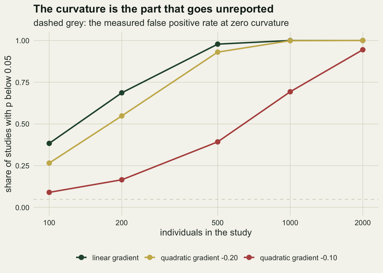
One trait at a time turns a saddle into disruptive selection
Now two traits, body size and flowering date, correlated with each other, on a fitness surface that has no curvature along either trait. The only nonlinear term is their product. Selection favours plants that are large and late, and plants that are small and early, and penalises the mismatched combinations. Nothing in the generating surface curves along the size axis alone.
n_pair   <- 4000
rho      <- 0.6
g12_true <- 0.30
mu_pair  <- 12

set.seed(8203)
z_size <- rnorm(n_pair)
z_time <- rho * z_size + sqrt(1 - rho^2) * rnorm(n_pair)
surf_pair <- 1 + g12_true * (z_size * z_time - rho)
off_pair  <- rpois(n_pair, mu_pair * pmax(surf_pair, 0.05))
w_pair    <- off_pair / mean(off_pair)
m_one   <- lm(w_pair ~ z_size + I(z_size^2))
g11_one <- 2 * unname(coef(m_one)[3])
t_one   <- summary(m_one)$coefficients[3, 3]
g11_pred <- 2 * rho * g12_true
The two traits are correlated at 0.60 and the correlational gradient is 0.30. Fitting size alone returns a quadratic gradient of 0.367 with a t value of 40. Read the way such a number is usually read, that is strong disruptive selection on body size, and the true gradient along the size axis is zero.
The size of the illusion is predictable. Regressing fitness on size alone integrates over flowering date, and for standardised traits the conditional mean of date given size is the correlation times size, so the product term contributes the correlational gradient times the correlation times z_size^2 to the fitted surface. Doubling that gives 0.36, and the fit returned 0.367. The apparent curvature is the correlational gradient multiplied by the trait correlation, counted twice: once through the conditional mean and once through the doubling.
The full quadratic model has both squared terms and the cross-product, and the gradients assemble into a matrix.
m_full <- lm(w_pair ~ z_size + z_time + I(z_size^2) + I(z_time^2) + z_size:z_time)
tab_full <- summary(m_full)$coefficients
cf_full <- coef(m_full)
sq_rows <- c("I(z_size^2)", "I(z_time^2)")
se_sq <- 2 * tab_full[sq_rows, 2]
t_sq  <- tab_full[sq_rows, 3]
p_sq  <- tab_full[sq_rows, 4]
t_12  <- tab_full["z_size:z_time", 3]

gam_mat <- matrix(c(2 * unname(cf_full["I(z_size^2)"]), unname(cf_full["z_size:z_time"]),
                    unname(cf_full["z_size:z_time"]), 2 * unname(cf_full["I(z_time^2)"])),
                  nrow = 2, dimnames = list(c("size", "date"), c("size", "date")))
eig_gam <- eigen(gam_mat)
axis1 <- eig_gam$vectors[, 1] * sign(eig_gam$vectors[1, 1])
axis2 <- eig_gam$vectors[, 2] * sign(eig_gam$vectors[1, 2])
ang1 <- atan2(axis1[2], axis1[1]) * 180 / pi
g11_full <- gam_mat[1, 1]
g22_full <- gam_mat[2, 2]
g12_full <- gam_mat[1, 2]
lam_up <- eig_gam$values[1]
lam_dn <- eig_gam$values[2]
The diagonal comes back at -0.019 for size, with a standard error of 0.011 and a t value of -1.69, and 0.004 for date, with a standard error of 0.010 and a t value of 0.46. Neither reaches the conventional threshold, at p values of 0.091 and 0.647, but the size term is close enough to it to be worth saying out loud: fitting the right model does not guarantee a clean zero on a term that is truly zero. The off-diagonal comes back at 0.305 against a generating value of 0.30, with a t value of 36. The cross-product coefficient is not doubled, for the reason given in the first section, and treating it as if it were would be the same error running the other way.
Phillips and Arnold (1989) made the case for going one step further and taking the eigenvalues of that matrix, because the squared terms on their own describe curvature along the axes the observer happened to measure, not along the axes the surface actually curves. Here the eigenvalues are +0.298 and -0.312, against a truth of plus and minus 0.30: one positive, one negative, which is a saddle. The positive axis lies at 46 degrees to the size axis, the combination of large and late, and along it fitness accelerates; along the perpendicular combination it falls away. The single-trait fit saw that positive eigenvalue, attributed all of it to body size, and returned a curvature 1.2 times the strongest curvature the true surface has in any direction.
one_dat <- bin_means(z_size, w_pair, half = 3)
one_line <- data.frame(z_size = seq(-3, 3, length.out = 200))
one_line$fit <- predict(m_one, one_line)

p_one <- ggplot(one_dat, aes(z, wbar)) +
  geom_point(size = 2.2, colour = te_ink) +
  geom_line(data = one_line, aes(z_size, fit), colour = te_rust, linewidth = 0.9) +
  labs(x = "body size (standardised)", y = "relative fitness",
       title = "Size alone", subtitle = "the U shape is not real") +
  theme_datasheet()

pred_grid <- expand.grid(z_size = seq(-2.6, 2.6, length.out = 90),
                         z_time = seq(-2.6, 2.6, length.out = 90))
pred_grid$w <- predict(m_full, pred_grid)
ax_end <- 2.4 * cbind(axis1, axis2)
seg_dat <- data.frame(x = -ax_end[1, ], y = -ax_end[2, ], xe = ax_end[1, ],
                      ye = ax_end[2, ],
                      axis_kind = c("positive eigenvalue", "negative eigenvalue"))

p_two <- ggplot(pred_grid, aes(z_size, z_time)) +
  geom_contour(aes(z = w, colour = after_stat(level)), linewidth = 0.5, bins = 14) +
  geom_segment(data = seg_dat, aes(x = x, y = y, xend = xe, yend = ye,
                                   linetype = axis_kind),
               colour = te_ink, linewidth = 0.6) +
  scale_colour_gradient(low = te_rust, high = te_forest, name = "fitted w") +
  scale_linetype_manual(values = c("positive eigenvalue" = "22",
                                   "negative eigenvalue" = "42"), name = NULL) +
  labs(x = "body size (standardised)", y = "flowering date (standardised)",
       title = "Both traits", subtitle = "hyperbolic contours: a saddle") +
  theme_datasheet()

p_one + p_two + plot_annotation(theme = theme_datasheet())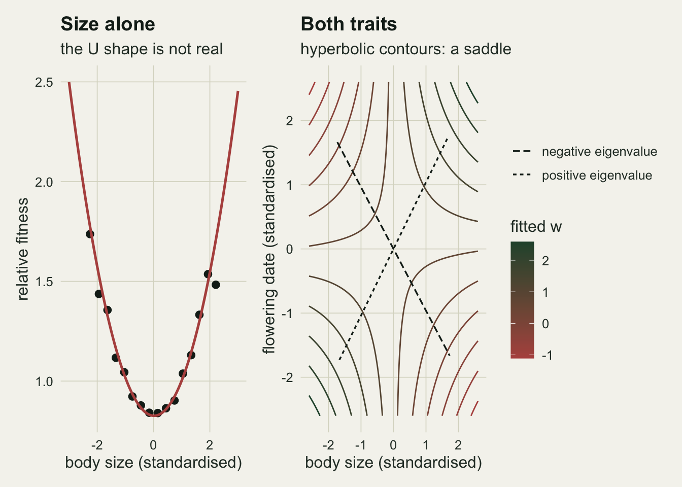
What to report
Say which convention the number is on. A quadratic selection gradient should be reported as twice the regression coefficient, and the sentence that says so belongs in the methods, because a reader cannot recover it from the table. If the coefficients are given as lm printed them, label them as coefficients and not as gradients. Report the whole gamma matrix, not the diagonal. Cross-product terms are gradients as fitted; squared terms need doubling; and the eigenvalues of the assembled matrix are what say whether the surface is a hill, a bowl or a saddle. A table of squared terms alone cannot be re-analysed by anyone.
Give the sample size next to the quadratic terms and resist the temptation to drop the ones that missed. A non-significant quadratic gradient at a hundred individuals carries almost no information about curvature, and reporting it with its standard error is more use to a later meta-analysis than reporting only the ones that cleared a threshold.
Standardise the traits and say how. Gradients on standardised traits are in units of phenotypic standard deviations and can be compared across studies; gradients on raw traits cannot. Mean standardised fitness is the other half of that convention. If a fitness surface width is quoted, give the trait variance and the directional gradient with it, and use both gradients to compute it. The width recovered from a gradient depends on the spread of the trait in the sample and on where the optimum sits relative to the trait mean; the short recipe that uses the quadratic gradient alone is the special case of a population already sitting on its optimum, and it is safe to assume only when the directional gradient is small enough that its square is negligible beside the quadratic one.
Honest limits
The quadratic model is a local approximation and nothing more. The first figure shows the fitted parabola leaving the true surface in the tails and eventually crossing below zero, which is not a possible fitness. Fitting a quadratic does not assert that the surface is a paraboloid; it asserts that a second-order expansion is a fair description over the range the data cover, and the further the traits spread the weaker that is. A cubic spline or a projection pursuit fit will show a surface the quadratic cannot, and the price is a set of numbers that no longer feed the multivariate breeder’s equation. The saddle diagnosed above has the same character: it lives in the space of the two traits that were measured, and an unmeasured trait correlated with both would rotate the eigenvectors and could change the sign of an eigenvalue, with no diagnostic within the data to reveal it.
The exact width formula used here holds for a Gaussian surface and a normally distributed trait. Both are assumptions. Skewed traits, truncation at a detection limit and fitness measured as survival rather than as a count all break the closed form, and the estimated gradient is then an average of curvature over an unknown weighting. The displaced optimum is different in kind from those three, because it does not break the closed form at all: it is inside it, and the section above shows what ignoring it costs. A field population with a modal optimum away from its trait mean is the normal case rather than the exception, and the width recipe that uses only the quadratic gradient is wrong there in a direction that flatters the analyst. The factor of two is unaffected by any of this: it is arithmetic, not a modelling assumption.
The detection experiment uses a single, simple generating model: one trait, Poisson offspring counts with a mean near replacement, and a fitness surface that is exactly quadratic. Real fitness data are more overdispersed than Poisson, which lowers detection further, and real studies often measure several traits, which spends degrees of freedom on cross-products faster than most sample sizes can afford. The detection rates here should be read as an optimistic ceiling. The generating surface is also floored at a small positive value to keep expected fitness non-negative, which changes the surface for a fraction 0.0056 of individuals at the stronger of the two generating gradients and less at the weaker one.
Fitness here is seed set or offspring count in a single episode. Lifetime fitness includes survival, and selection through one episode can be reversed by another. Blows and Brooks (2003) make the wider point that nonlinear selection estimated from a small number of traits is routinely reported as if it described the surface, when the number of dimensions any study can support is smaller than the number of traits that matter.
References
Lande R, Arnold SJ 1983 Evolution 37(6):1210-1226 (10.1111/j.1558-5646.1983.tb00236.x)
Stinchcombe JR, Agrawal AF, Hohenlohe PA, Arnold SJ, Blows MW 2008 Evolution 62(9):2435-2440 (10.1111/j.1558-5646.2008.00449.x)
Kingsolver JG, Hoekstra HE, Hoekstra JM, Berrigan D, Vignieri SN, Hill CE, Hoang A, Gibert P, Beerli P 2001 The American Naturalist 157(3):245-261 (10.1086/319193)
Phillips PC, Arnold SJ 1989 Evolution 43(6):1209-1222 (10.1111/j.1558-5646.1989.tb02569.x)
Blows MW, Brooks R 2003 The American Naturalist 162(6):815-820 (10.1086/378905)