library(ggplot2)
library(nlme)

te_paper  <- "#f5f4ee"
te_ink    <- "#16241d"
te_body   <- "#2c3a31"
te_forest <- "#275139"
te_rust   <- "#b5534e"
te_gold   <- "#c9b458"
te_line   <- "#dad9ca"

theme_datasheet <- function() {
  theme_minimal(base_size = 12) +
    theme(plot.background  = element_rect(fill = te_paper, colour = NA),
          panel.background = element_rect(fill = te_paper, colour = NA),
          panel.grid.major = element_line(colour = te_line, linewidth = 0.3),
          panel.grid.minor = element_blank(),
          text             = element_text(colour = te_body),
          plot.title       = element_text(colour = te_ink, face = "bold"),
          plot.subtitle    = element_text(colour = te_body),
          axis.text        = element_text(colour = te_body))
}Nonlinear selection on BLUPs and on raw means
R
selection gradients
mixed models
measurement error
behavioural ecology
simulation
ecology tutorial
When assay counts track lifespan, BLUPs fake disruptive selection and raw means fake stabilising selection. Quadratic selection gradients simulated in R.
Every spring a field team walks a boulder field, catches the marked lizards it can find, and runs each one through a five minute open-field test scored from video. A lizard caught in its first spring and never again has one test. One that lives six years and is found in four of them has four. At the end of the study there is an exploration score for every animal, a count of hatchlings assigned to each by parentage, and a question in the grant: is exploration under stabilising or disruptive selection?
The usual route has two steps. The first is a repeatability model, a random intercept for the animal fitted to all the tests. The second takes each animal’s predicted intercept, its BLUP, standardises it, and puts it into a Lande-Arnold regression of relative lifetime success on the score and its square. Twice the coefficient of the square is the quadratic selection gradient, and its sign says which kind of selection it is.
That second step is a known misuse, and this post is a demonstration of it, not a claim to it. Postma (2006) set out how predicted breeding values differ from true ones and what the difference does to their relationship with fitness. Hadfield and colleagues (2010) showed analytically and by simulation that BLUPs carried into a second analysis give biased estimates and standard errors that are far too small. Houslay and Wilson (2017) carried the warning into behavioural ecology, where the predicted intercepts of a repeatability model are exactly what gets correlated with fitness, and recommended fitting the relationship inside a bivariate mixed model instead; that model estimates a covariance between behaviour and fitness, which is linear selection, and has no term for curvature. What is measured here is narrower: what the quadratic gradient does when the number of assays an animal gets is set by how long it lives, as it is in any study that assays animals opportunistically at recapture, and which of the obvious repairs actually repair it.
The animal model in R builds BLUPs from a pedigree and shows that the set of predictions is narrower than the truth, which is why it calls feeding them to a second analysis dangerous; it names the danger and runs no second analysis. Measurement error and regression dilution treats classical error, which by construction does not depend on the response, and closes on the rule that attenuation cannot manufacture an effect, only weaken a real one. The case below is the other one. The error variance of each animal’s score depends on how long it lived, and so on its fitness, and it manufactures curvature where there is none.
The nearest design problem on the site is per chick or per nest, where the number of measurements per unit also carries information about the outcome and the repair is to analyse one row per nest. Here each animal is already one row and counts once, and the analysis still fails, because what depends on the count is not the weight of the animal but the spread of its score. Nonlinear selection gradients in R covers the doubling of the squared coefficient and how hard curvature is to detect even when the trait is measured exactly; every gradient below is on its doubled convention. Checking a selection analysis already makes the point that count fitness breaks the ordinary least squares standard error, and that half of the repair is used here, not claimed.
The spread of a score depends on how many assays it averages
Take the among-individual variance of the behaviour as 0.37 and the within-individual variance as 0.63, so that the repeatability is 0.37, the average across the behavioural literature in the meta-analysis by Bell and colleagues (2009). An animal assayed n times has a raw mean whose variance about the population mean is the among-individual variance plus the assay variance divided by n. Its BLUP is that deviation multiplied by the reliability, the among-individual variance divided by the variance of the mean, so its expected square is the among-individual variance times the reliability. The prediction error variance (PEV) is what the BLUP leaves out, and the sum of the squared BLUP and the PEV is the conditional expectation of the squared true value given the data. It is not the square of the best prediction; it is the best prediction of the square.
va_true <- 0.37                      # among-individual variance of the behaviour
ve_true <- 0.63                      # within-individual (assay) variance
n_tab  <- 1:8
rel_n  <- n_tab * va_true / (n_tab * va_true + ve_true)
mom_tab <- data.frame(n_assays = n_tab,
                      reliability = rel_n,
                      blup_sq = va_true * rel_n,
                      mean_sq = va_true + ve_true / n_tab,
                      calibrated = va_true * rel_n + va_true * (1 - rel_n))
print(round(mom_tab, 3), row.names = FALSE)
n_assays reliability blup_sq mean_sq calibrated
1 0.370 0.137 1.000 0.37
2 0.540 0.200 0.685 0.37
3 0.638 0.236 0.580 0.37
4 0.701 0.260 0.527 0.37
5 0.746 0.276 0.496 0.37
6 0.779 0.288 0.475 0.37
7 0.804 0.298 0.460 0.37
8 0.825 0.305 0.449 0.37# a check by simulation, with the variances known
n_check <- 20000
set.seed(32701)
mom_sim <- do.call(rbind, lapply(n_tab, function(k) {
a_k <- rnorm(n_check, 0, sqrt(va_true))
ybar <- a_k + rnorm(n_check, 0, sqrt(ve_true / k))
rel_k <- k * va_true / (k * va_true + ve_true)
blup <- rel_k * ybar
pev_k <- va_true * (1 - rel_k)
data.frame(n_assays = k, blup_sq = mean(blup^2), mean_sq = mean(ybar^2),
calibrated = mean(blup^2 + pev_k))
}))
mom_gap <- max(abs(as.matrix(mom_sim[, -1]) -
as.matrix(mom_tab[, c("blup_sq", "mean_sq", "calibrated")])))The expected squared BLUP rises from 0.137 for an animal with one assay to 0.305 for one with eight. The expected squared raw mean falls over the same range from 1.000 to 0.449. The squared BLUP plus PEV is 0.37 at every assay count. A simulation with 20000 animals per count and the variances known lands within 0.009 of the closed form everywhere.
That table predicts the sign of both biases without any simulation of fitness. Under no selection on the behaviour, animals that live longer have more offspring and more assays. Their BLUPs are spread wider than those of short-lived animals, so the animals at the two ends of the BLUP axis are disproportionately long-lived and successful, and a parabola fitted through them opens upward: disruptive selection. Their raw means are spread narrower, so the ends of the raw-mean axis belong to short-lived animals with a single assay and little success, and the parabola opens downward: stabilising selection. Shrinkage decides which sign appears. The cause is that the precision of the score depends on the outcome, and only the size of each bias needs the simulation that follows.
mom_long <- data.frame(
  n_assays = rep(n_tab, 3),
  value = c(mom_tab$blup_sq, mom_tab$mean_sq, mom_tab$calibrated),
  sim = c(mom_sim$blup_sq, mom_sim$mean_sq, mom_sim$calibrated),
  summary = rep(c("squared BLUP", "squared raw mean", "squared BLUP plus PEV"),
                each = length(n_tab)))
mom_long$summary <- factor(mom_long$summary,
                           levels = c("squared raw mean", "squared BLUP plus PEV", "squared BLUP"))
ggplot(mom_long, aes(n_assays, value, colour = summary)) +
  geom_hline(yintercept = va_true, linetype = "dashed", colour = te_ink, linewidth = 0.4) +
  geom_line(linewidth = 0.9) +
  geom_point(aes(y = sim), size = 2.4, shape = 21, fill = te_paper, stroke = 1) +
  scale_colour_manual(values = c(te_rust, te_gold, te_forest), name = NULL) +
  scale_x_continuous(breaks = n_tab) +
  labs(x = "assays of the animal", y = "expected square of the summary",
       title = "The spread of a summary depends on its assay count",
       subtitle = "lines: closed form; open circles: simulation; dashed: the among-individual variance") +
  theme_datasheet() +
  theme(legend.position = "bottom")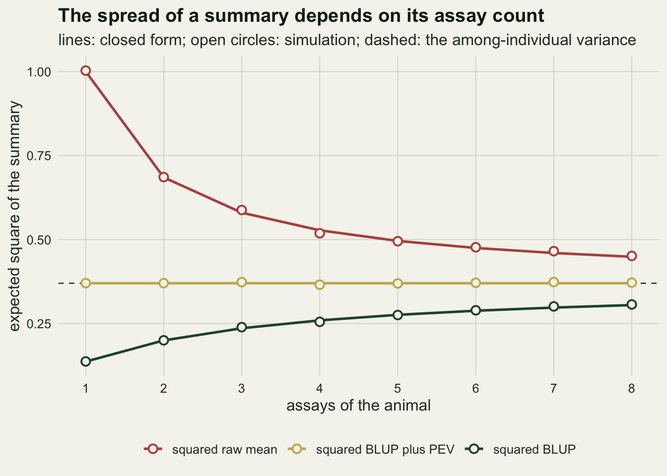
One population, two opposite surfaces
The generator follows one cohort of 150 animals. Annual survival is 0.55 and the years alive are one plus a geometric count, capped at ten. Every animal is assayed in its first year, and in each later year alive it is found and assayed with probability 0.6. Lifetime reproductive success is negative binomial with size 1.5 and a mean of 1.2 offspring per year alive. In this section the behaviour has no effect on survival or on reproduction at all.
The repeatability model is a one-way random intercept fitted by REML. Fitting it thousands of times with nlme is slow, so the code below profiles the ratio of the two variances with optimize, which for this model gives the REML estimates, the BLUPs and the plug-in PEV in closed form. The agreement check that follows compares it with nlme::lme on fresh data sets.
s_annual <- 0.55                     # annual survival
life_cap <- 10                       # oldest possible age in years
lrs_per_year <- 1.2                  # mean offspring per year alive
nb_size  <- 1.5                      # negative binomial size of lifetime success
va_floor <- 0.05                     # boundary guard on the estimated variance

gen_pop <- function(n_anim, sel = "none", assay = "prob", p_assay = 0.6,
                    shuffle = 0, fit_dist = "nb") {
  a_i  <- rnorm(n_anim, 0, sqrt(va_true))
  z_i  <- a_i / sqrt(va_true)
  surv <- rep(s_annual, n_anim)
  if (sel == "via") surv <- plogis(qlogis(s_annual) - 0.25 * (z_i^2 - 1))
  years <- pmin(1 + rgeom(n_anim, 1 - surv), life_cap)
  n_id <- switch(assay,
                 prob  = 1L + rbinom(n_anim, years - 1, p_assay),
                 every = as.integer(years),
                 fixed = rep(3L, n_anim))
  if (shuffle > 0) {
    k_mix <- sample(n_anim, round(shuffle * n_anim))
    n_id[k_mix] <- n_id[k_mix][sample(length(k_mix))]
  }
  mu_w <- lrs_per_year * years
  if (sel == "fec") mu_w <- mu_w * exp(-0.3 / 2 * (z_i^2 - 1))
  lrs <- if (fit_dist == "pois") rpois(n_anim, mu_w) else
    rnbinom(n_anim, size = nb_size, mu = mu_w)
  list(a = a_i, n_id = n_id, lrs = lrs)
}

# one-way REML by profiling the variance ratio; BLUP and plug-in PEV
reml_oneway <- function(y, id, n_id) {
  n_obs <- length(y)
  ybar  <- as.numeric(rowsum(y, id)) / n_id
  ssw   <- sum((y - ybar[id])^2)
  prof  <- function(log_lam) {
    lam <- exp(log_lam); c_i <- n_id / (1 + n_id * lam)
    mu  <- sum(c_i * ybar) / sum(c_i)
    q   <- ssw + sum(c_i * (ybar - mu)^2)
    (n_obs - 1) * log(q / (n_obs - 1)) + sum(log(1 + n_id * lam)) + log(sum(c_i))
  }
  lam <- exp(optimize(prof, c(-9, 4), tol = 1e-8)$minimum)
  c_i <- n_id / (1 + n_id * lam)
  mu  <- sum(c_i * ybar) / sum(c_i)
  ve  <- (ssw + sum(c_i * (ybar - mu)^2)) / (n_obs - 1)
  va  <- lam * ve
  list(va = va, ve = ve, mu = mu, ybar = ybar,
       blup = n_id * lam / (1 + n_id * lam) * (ybar - mu),
       pev = va * ve / (ve + n_id * va))
}

# gradient = twice the squared-term coefficient; p values from OLS and HC3
quad_fit <- function(w, x1, x2, extra = NULL) {
  X    <- cbind(1, x1, x2, extra)
  XtXi <- solve(crossprod(X))
  b    <- XtXi %*% crossprod(X, w)
  e    <- as.numeric(w - X %*% b)
  h    <- rowSums((X %*% XtXi) * X)
  df_r <- length(w) - ncol(X)
  se_ols <- sqrt(XtXi[3, 3] * sum(e^2) / df_r)
  v_hc3  <- XtXi %*% crossprod(X * (e / (1 - h))) %*% XtXi
  c(g = 2 * b[3], p_ols = 2 * pt(-abs(b[3] / se_ols), df_r),
    p_hc3 = 2 * pt(-abs(b[3] / sqrt(v_hc3[3, 3])), df_r))
}

std <- function(x) (x - mean(x)) / sd(x)

# the first assay of every animal, calibrated with the variances given
first_fit <- function(w, y1, va, ve, mu) {
  rel1 <- va / (va + ve)
  b1   <- rel1 * (y1 - mu)
  quad_fit(w, b1 / sqrt(va), (b1^2 + va * (1 - rel1)) / va)
}

# moment variances: the first assays estimate va + ve, the repeat assays ve
first_moments <- function(y, id, ybar, n_id) {
  y1  <- y[!duplicated(id)]
  ve1 <- sum((y - ybar[id])^2) / (length(y) - length(n_id))
  list(y1 = y1, va = var(y1) - ve1, ve = ve1, mu = mean(y1))
}

# five analyses of the same data set
arms_of <- function(pop, y, id, f) {
  w  <- pop$lrs / mean(pop$lrs)
  zb <- std(f$blup); zr <- std(f$ybar)
  m1 <- first_moments(y, id, f$ybar, pop$n_id)
  no_n <- c(g = NA, p_ols = NA, p_hc3 = NA)
  c(blup  = quad_fit(w, zb, zb^2),
    raw   = quad_fit(w, zr, zr^2),
    cal   = quad_fit(w, f$blup / sqrt(f$va), (f$blup^2 + f$pev) / f$va),
    logn  = if (var(pop$n_id) > 0) quad_fit(w, zb, zb^2, log(pop$n_id)) else no_n,
    first = if (m1$va >= va_floor) first_fit(w, m1$y1, m1$va, m1$ve, m1$mu) else no_n,
    va = f$va, va1 = m1$va,
    cor_nw = if (var(pop$n_id) > 0) cor(pop$n_id, pop$lrs) else 0,
    mean_n = mean(pop$n_id))
}

one_rep <- function(n_anim, sel, assay, p_assay, shuffle, fit_dist) {
  pop <- gen_pop(n_anim, sel, assay, p_assay, shuffle, fit_dist)
  id  <- rep(seq_len(n_anim), pop$n_id)
  y   <- pop$a[id] + rnorm(length(id), 0, sqrt(ve_true))
  arms_of(pop, y, id, reml_oneway(y, id, pop$n_id))
}
n_agree <- 20
set.seed(32702)
agree <- t(replicate(n_agree, {
pop <- gen_pop(150)
id <- rep(seq_len(150), pop$n_id)
y <- pop$a[id] + rnorm(length(id), 0, sqrt(ve_true))
f <- reml_oneway(y, id, pop$n_id)
fit <- lme(y ~ 1, random = ~ 1 | id, method = "REML",
data = data.frame(y = y, id = factor(id)))
vc <- as.numeric(VarCorr(fit)[, "Variance"])
c(va = abs(f$va - vc[1]) / vc[1], ve = abs(f$ve - vc[2]) / vc[2],
blup = max(abs(f$blup - ranef(fit)[, 1])))
}))
agree_max <- apply(agree, 2, max)
print(signif(agree_max, 2)) va ve blup
2.1e-06 8.0e-07 1.7e-06 Over 20 data sets the largest relative difference from lme is \(2.1 \times 10^{-6}\) in the among-individual variance and \(8.0 \times 10^{-7}\) in the residual variance, and the largest difference in any BLUP is \(1.7 \times 10^{-6}\). The two are the same fit.
The five analyses run on each data set are the two field versions, the standardised BLUP and the standardised raw mean, and three repairs. The calibrated square regresses fitness on the BLUP and on the squared BLUP plus PEV, both divided by the estimated among-individual variance so that the gradient is per standard deviation of the true value. The second repair is the one most people reach for, the standardised BLUP with the log of the assay count as a covariate. The third uses only the first assay of each animal, the one every animal has, so that every animal’s score has the same precision whatever its fate. It is calibrated in the same way, but with variances estimated by moments instead of taken from the REML fit: the variance of the first assays estimates the among-individual plus the within-individual variance, the pooled variance of the repeat assays about each animal’s own mean estimates the within-individual part, and the difference is the among-individual variance. Why the REML estimates are not used here shows up under viability selection.
n_work <- 150
set.seed(32703)
pop_w <- gen_pop(n_work)
id_w  <- rep(seq_len(n_work), pop_w$n_id)
y_w   <- pop_w$a[id_w] + rnorm(length(id_w), 0, sqrt(ve_true))
fit_w <- lme(y ~ 1, random = ~ 1 | id, method = "REML",
             data = data.frame(y = y_w, id = factor(id_w)))
vc_w  <- as.numeric(VarCorr(fit_w)[, "Variance"])
f_w   <- reml_oneway(y_w, id_w, pop_w$n_id)
arm_w <- arms_of(pop_w, y_w, id_w, f_w)
w_w   <- pop_w$lrs / mean(pop_w$lrs)
n_single <- sum(pop_w$n_id == 1)
cor_w <- cor(pop_w$n_id, pop_w$lrs)
sd_by_n <- data.frame(
  group = c("one assay", "four or more"),
  sd_blup = c(sd(f_w$blup[pop_w$n_id == 1]), sd(f_w$blup[pop_w$n_id >= 4])),
  sd_raw  = c(sd(f_w$ybar[pop_w$n_id == 1]), sd(f_w$ybar[pop_w$n_id >= 4])),
  mean_w  = c(mean(w_w[pop_w$n_id == 1]), mean(w_w[pop_w$n_id >= 4])),
  animals = c(sum(pop_w$n_id == 1), sum(pop_w$n_id >= 4)))
print(round(c(animals = n_work, assays = length(y_w), single = n_single,
              va_hat = vc_w[1], ve_hat = vc_w[2], cor_n_lrs = cor_w,
              g_blup = unname(arm_w["blup.g"]), g_raw = unname(arm_w["raw.g"]),
              g_cal = unname(arm_w["cal.g"])), 3))
animals assays single va_hat ve_hat cor_n_lrs g_blup g_raw
150.000 288.000 80.000 0.361 0.692 0.476 0.104 -0.219
g_cal
-0.041 print(sd_by_n, digits = 3, row.names = FALSE) group sd_blup sd_raw mean_w animals
one assay 0.373 1.09 0.569 80
four or more 0.552 0.79 2.223 21One data set shows the whole problem. The 150 animals received 288 assays between them and 80 were assayed once. lme puts the among-individual variance at 0.361 and the residual at 0.692, and the correlation between assay count and lifetime success is 0.476. The quadratic gradient on the standardised BLUPs is +0.104, on the standardised raw means -0.219, and on the calibrated square -0.041: disruptive selection, stabilising selection and very little, from one set of numbers with no selection in it.
The mechanism is visible in two rows of the data. The 80 single-assay animals have a mean relative success of 0.57, their BLUPs have a standard deviation of 0.373 and their raw means 1.09. The 21 animals with four or more assays have a mean relative success of 2.22, BLUPs spread to 0.552 and raw means narrowed to 0.79.
x_grid <- seq(-3, 3, length.out = 121)
curve_of <- function(x) {
  cf <- coef(lm(w_w ~ x + I(x^2)))
  cf[1] + cf[2] * x_grid + cf[3] * x_grid^2
}
zb_w <- std(f_w$blup); zr_w <- std(f_w$ybar)
pts_w <- data.frame(x = c(zb_w, zr_w), w = rep(w_w, 2),
                    arm = rep(c("BLUP", "raw mean"), each = n_work))
crv_w <- data.frame(x = rep(x_grid, 2), w = c(curve_of(zb_w), curve_of(zr_w)),
                    arm = rep(c("BLUP", "raw mean"), each = length(x_grid)))
ggplot(pts_w, aes(x, w, colour = arm)) +
  geom_point(size = 1.3, alpha = 0.45) +
  geom_line(data = crv_w, linewidth = 1.1) +
  scale_colour_manual(values = c("BLUP" = te_forest, "raw mean" = te_rust), name = NULL) +
  coord_cartesian(xlim = c(-3, 3), ylim = c(0, max(w_w) + 0.1)) +
  labs(x = "behaviour score, standardised", y = "relative lifetime success",
       title = "One data set, two fitness surfaces",
       subtitle = "no selection on the behaviour; curves are the Lande-Arnold quadratic fits") +
  theme_datasheet() +
  theme(legend.position = "bottom")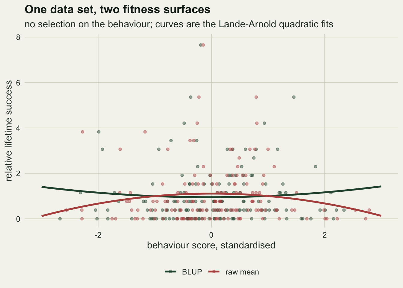
The link, not the shrinkage
One data set is one draw. The scenarios below each run five independent draws of 1000 replicate studies, and every gradient reported is the median over the five draws of the mean over a draw’s replicates, with the range over draws beside it. Four scenarios have no selection: the design above; one where every animal is assayed in every year it is alive and success is Poisson, which makes the link between assay count and success the tightest this generator allows; one where the assay counts are shuffled among animals, so that each animal keeps a realistic count but the count no longer follows its fate; and one where every animal is assayed exactly three times. Replicates whose estimated among-individual variance falls below 0.05 are dropped from every analysis, because the calibrated square divides by it; the count dropped is printed with the table. The first-assay repair divides by its own moment estimate, and it also skips the replicates where that estimate falls below the guard.
cells <- data.frame(
  name = c("null", "null, every year assayed", "null, counts shuffled",
           "null, three assays each", "fecundity selection", "viability selection",
           "fecundity, three assays each"),
  sel = c("none", "none", "none", "none", "fec", "via", "fec"),
  assay = c("prob", "every", "prob", "fixed", "prob", "prob", "fixed"),
  shuffle = c(0, 0, 1, 0, 0, 0, 0),
  fit_dist = c("nb", "pois", "nb", "nb", "nb", "nb", "nb"))
n_draw <- 5; n_per <- 1000; n_anim <- 150
arm_names <- c("blup", "raw", "cal", "logn", "first")

run_cell <- function(n_anim, sel, assay, p_assay, shuffle, fit_dist, reps, seed0) {
  lapply(seq_len(n_draw), function(d) {
    set.seed(seed0 + d)
    t(replicate(reps, one_rep(n_anim, sel, assay, p_assay, shuffle, fit_dist)))
  })
}
cell_summary <- function(draws) {
  kept <- lapply(draws, function(m) m[m[, "va"] >= va_floor, , drop = FALSE])
  gcol <- paste0(arm_names, ".g")
  gm <- sapply(kept, function(m) colMeans(m[, gcol, drop = FALSE], na.rm = TRUE))
  pooled <- do.call(rbind, kept)
  n_ok <- colSums(!is.na(pooled[, gcol]))
  data.frame(arm = arm_names,
             g_med = apply(gm, 1, median), g_lo = apply(gm, 1, min), g_hi = apply(gm, 1, max),
             g_sd = apply(pooled[, gcol], 2, sd, na.rm = TRUE),
             g_se = apply(pooled[, gcol], 2, sd, na.rm = TRUE) / sqrt(n_ok),
             rej_ols = colMeans(pooled[, paste0(arm_names, ".p_ols")] < 0.05, na.rm = TRUE),
             rej_hc3 = colMeans(pooled[, paste0(arm_names, ".p_hc3")] < 0.05, na.rm = TRUE),
             cor_nw = mean(pooled[, "cor_nw"]), mean_n = mean(pooled[, "mean_n"]),
             kept = n_ok, dropped = n_draw * nrow(draws[[1]]) - nrow(pooled),
             dropped_first = sum(is.na(pooled[, "first.g"])))
}
scen_res <- lapply(seq_len(nrow(cells)), function(k) {
  s <- cell_summary(run_cell(n_anim, cells$sel[k], cells$assay[k], 0.6, cells$shuffle[k],
                             cells$fit_dist[k], n_per, 32710 + 100 * k))
  cbind(cell = cells$name[k], s)
})
scen_tab <- do.call(rbind, scen_res); rownames(scen_tab) <- NULL

# oracle: the quadratic gradient of relative fitness on the true standardised value
n_oracle <- 2e5
set.seed(32790)
oracle <- sapply(c("fec", "via"), function(s) {
  pop <- gen_pop(n_oracle, sel = s)
  z <- pop$a / sqrt(va_true); w <- pop$lrs / mean(pop$lrs)
  fo <- summary(lm(w ~ z + I(z^2)))$coefficients
  c(g = 2 * fo[3, 1], se = 2 * fo[3, 2])
})
print(scen_tab[, c("cell", "arm", "g_med", "g_lo", "g_hi", "g_se", "rej_ols", "rej_hc3",
                   "cor_nw", "dropped")], digits = 3, row.names = FALSE)
cell arm g_med g_lo g_hi g_se
null blup 0.152241 0.143340 0.15365 0.00271
null raw -0.123613 -0.128353 -0.11495 0.00187
null cal -0.013334 -0.031458 -0.00348 0.00653
null logn -0.000317 -0.008199 0.00540 0.00250
null first 0.009319 -0.005198 0.03661 0.00794
null, every year assayed blup 0.176498 0.172538 0.17914 0.00173
null, every year assayed raw -0.151724 -0.154795 -0.14988 0.00126
null, every year assayed cal -0.020646 -0.027898 -0.01642 0.00374
null, every year assayed logn -0.003631 -0.004412 -0.00156 0.00126
null, every year assayed first 0.002468 -0.000617 0.01069 0.00521
null, counts shuffled blup 0.002467 -0.003978 0.00721 0.00232
null, counts shuffled raw 0.001226 -0.006761 0.00640 0.00233
null, counts shuffled cal 0.008676 -0.012508 0.01585 0.00545
null, counts shuffled logn 0.002520 -0.004880 0.00792 0.00236
null, counts shuffled first 0.004464 -0.036157 0.02424 0.00797
null, three assays each blup 0.003176 -0.003116 0.00549 0.00236
null, three assays each raw 0.003176 -0.003116 0.00549 0.00236
null, three assays each cal 0.005284 -0.004770 0.00950 0.00377
null, three assays each logn NA NaN NaN NA
null, three assays each first -0.004335 -0.006063 0.01906 0.00723
fecundity selection blup 0.015934 0.009376 0.02571 0.00233
fecundity selection raw -0.217118 -0.219665 -0.21397 0.00168
fecundity selection cal -0.335163 -0.339493 -0.31767 0.00590
fecundity selection logn -0.138159 -0.140561 -0.13622 0.00219
fecundity selection first -0.241299 -0.246824 -0.20728 0.00717
viability selection blup 0.077900 0.069280 0.08160 0.00257
viability selection raw -0.197077 -0.201576 -0.19148 0.00164
viability selection cal -0.341638 -0.355815 -0.31735 0.00782
viability selection logn -0.029199 -0.036515 -0.02329 0.00231
viability selection first -0.182124 -0.189372 -0.16841 0.00747
fecundity, three assays each blup -0.148163 -0.150181 -0.14397 0.00198
fecundity, three assays each raw -0.148163 -0.150181 -0.14397 0.00198
fecundity, three assays each cal -0.234733 -0.235980 -0.22614 0.00317
fecundity, three assays each logn NA NaN NaN NA
fecundity, three assays each first -0.249977 -0.251005 -0.23584 0.00645
rej_ols rej_hc3 cor_nw dropped
0.1995 0.0694 4.59e-01 3
0.0568 0.1997 4.59e-01 3
0.0947 0.0638 4.59e-01 3
0.0999 0.0580 4.59e-01 3
0.0477 0.0627 4.59e-01 3
0.3809 0.2505 7.62e-01 1
0.2488 0.4247 7.62e-01 1
0.0904 0.0454 7.62e-01 1
0.0916 0.0490 7.62e-01 1
0.0508 0.0596 7.62e-01 1
0.0538 0.0692 2.76e-05 1
0.0536 0.0660 2.76e-05 1
0.0530 0.0658 2.76e-05 1
0.0530 0.0664 2.76e-05 1
0.0520 0.0697 2.76e-05 1
0.0488 0.0668 0.00e+00 0
0.0488 0.0668 0.00e+00 0
0.0488 0.0668 0.00e+00 0
NaN NaN 0.00e+00 0
0.0464 0.0652 0.00e+00 0
0.0616 0.0622 4.51e-01 1
0.1968 0.4623 4.51e-01 1
0.1442 0.1790 4.51e-01 1
0.1732 0.2030 4.51e-01 1
0.0468 0.1406 4.51e-01 1
0.1056 0.0497 4.72e-01 30
0.1475 0.4135 4.72e-01 30
0.1380 0.1388 4.72e-01 30
0.0761 0.0678 4.72e-01 30
0.0389 0.1219 4.72e-01 30
0.0854 0.2644 0.00e+00 0
0.0854 0.2644 0.00e+00 0
0.0854 0.2644 0.00e+00 0
NaN NaN 0.00e+00 0
0.0432 0.1437 0.00e+00 0print(round(oracle, 4)) fec via
g -0.2330 -0.1899
se 0.0044 0.0044gv <- function(cell, arm, col = "g_med") scen_tab[scen_tab$cell == cell & scen_tab$arm == arm, col]
g_kingsolver <- 0.10 # compiled median absolute quadratic gradient, Kingsolver et al. 2001
null_gap <- gv("null", "blup") - gv("null", "raw")
rel_three <- 3 * va_true / (3 * va_true + ve_true)In the design above, the standardised BLUP returns a quadratic gradient of +0.152 (draws +0.143 to +0.154) and the standardised raw mean -0.124 (-0.128 to -0.115), with a mean correlation between assay count and success of 0.46. The three repairs sit at -0.013 for the calibrated square, -0.0003 with log assay count as a covariate and +0.009 for the first assay. Only 3 of the 5000 replicates fell below the variance guard, and the moment estimate behind the first assay fell below it in a further 33. When every year is assayed the correlation rises to 0.76 and the two field gradients move apart, to +0.176 and -0.152.
The two controls settle the cause. With the same assay counts shuffled among animals, every analysis falls to between +0.001 and +0.009. The distribution of shrinkage is exactly as before, and the bias has gone, because the shrinkage no longer lines up with fitness. With three assays each, every BLUP is shrunk by the same factor, standardising removes it, and the BLUP and raw-mean gradients are identical at +0.003.
The gap between the two field answers under no selection is 0.276. The compilation by Kingsolver and colleagues (2001) put the median absolute quadratic gradient in published studies at 0.10, which makes the gap 2.8 times a typical reported curvature. The nonlinear gradients post explains why that median may understate the doubled gradient by as much as a factor of two; against a median of 0.20 the gap is still 1.4 times it.
When selection is real
Two selection scenarios use the same design. In the first, stabilising selection acts on fecundity: the expected number of offspring per year alive falls as the squared standardised behaviour rises, and survival is untouched. In the second, the same kind of selection acts on survival instead, so that animals far from the mean die younger, which means their assay counts depend on their behaviour as well as on their luck. The target is an oracle gradient: the quadratic gradient of relative success on the true standardised value, from one population of 200000 animals, -0.233 for fecundity selection and -0.190 for viability selection, with standard errors of 0.004 and 0.004.
arm_lab <- c(blup = "BLUP", raw = "raw mean", cal = "BLUP squared plus PEV",
             logn = "BLUP with log(n)", first = "first assay, moment variances")
plot_tab <- scen_tab[!is.na(scen_tab$g_med), ]
plot_tab$arm_f <- factor(arm_lab[plot_tab$arm], levels = rev(arm_lab))
plot_tab$cell_f <- factor(plot_tab$cell, levels = cells$name)
ref_tab <- data.frame(cell_f = factor(cells$name, levels = cells$name),
                      g = c(0, 0, 0, 0, oracle["g", "fec"], oracle["g", "via"], oracle["g", "fec"]))
ggplot(plot_tab, aes(g_med, arm_f, colour = arm, shape = arm)) +
  geom_vline(data = ref_tab, aes(xintercept = g), linetype = "dashed",
             colour = te_ink, linewidth = 0.4) +
  geom_errorbar(aes(xmin = g_lo, xmax = g_hi), orientation = "y", width = 0, linewidth = 0.8) +
  geom_point(size = 2.4) +
  facet_wrap(~ cell_f, ncol = 2) +
  scale_colour_manual(values = c(blup = te_forest, raw = te_rust, cal = te_gold,
                                 logn = te_body, first = te_ink), guide = "none") +
  scale_shape_manual(values = c(blup = 16, raw = 16, cal = 16, logn = 15, first = 17),
                     guide = "none") +
  labs(x = "quadratic selection gradient (median of five draws, bar: range)", y = NULL,
       title = "Where each analysis lands",
       subtitle = "dashed: zero under no selection, the oracle gradient under selection") +
  theme_datasheet() +
  theme(strip.text = element_text(colour = te_ink, face = "bold"))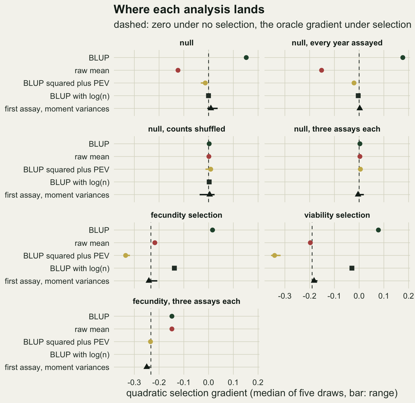
Under fecundity selection the standardised BLUP reads +0.016: the spurious disruptive term has cancelled the real stabilising one and the selection is gone. Under viability selection it reads +0.078, the wrong sign. The raw mean lands at -0.217 and -0.197, close to both oracles, and that closeness is a coincidence of two errors: a spurious stabilising term like the one measured under no selection, plus a real gradient shrunk by the noise in single-assay means. In the design with three assays each, where there is no link, the same raw mean reads -0.148 under fecundity selection. That is the oracle times the reliability of a three-assay mean, 0.638 times -0.233, or -0.149, which is what a standardised noisy predictor does to a quadratic gradient; it is also why the BLUP and raw-mean gradients in the figure are per standard deviation of their own scores and not of the truth.
The covariate repair behaves as its logic predicts. Adding log assay count removes the null bias, but under fecundity selection it returns -0.138, still per standard deviation of a shrunken score, and under viability selection it returns -0.029. When the behaviour kills the animal, how many assays it had is part of the selection, and conditioning on the count conditions most of the selection away.
The calibrated square has the right sign in both scenarios and overshoots in both: -0.335 against an oracle of -0.233, and -0.342 against -0.190. It is not a flaw in the calibration itself: with three assays each it returns -0.235. The overshoot is the same link again, acting on a different quantity. A regression on the calibrated square averages the curvature over animals in proportion to how much their calibrated squares vary, and that spread grows with the assay count, so the long-lived animals dominate the fit. Long-lived animals also hold more of the population’s offspring, since success scales with years alive, and in relative-fitness units their curvature is larger. The weighting can be written down and checked.
set.seed(32840)
pop_big <- gen_pop(4e5, sel = "fec")
share_n <- table(pop_big$n_id) / length(pop_big$n_id)
n_vals  <- as.numeric(names(share_n))
lrs_n   <- as.numeric(tapply(pop_big$lrs, pop_big$n_id, mean))
rel_v   <- n_vals * va_true / (n_vals * va_true + ve_true)
# the calibrated square has variance proportional to rel^2 within a count class
infl_pred <- sum(share_n * rel_v^2 * lrs_n) / (mean(pop_big$lrs) * sum(share_n * rel_v^2))
print(round(c(inflation = infl_pred, predicted = infl_pred * oracle["g", "fec"],
              measured = gv("fecundity selection", "cal")), 3))
inflation predicted measured
1.344 -0.313 -0.335 Within an assay-count class, the variance of the calibrated square is proportional to the squared reliability, and under fecundity selection the curvature within a class scales with that class’s mean success. Weighting the class means of success by the class shares times the squared reliability, and dividing by the plain population mean, predicts an inflation of 1.34, a calibrated gradient of -0.313 against the -0.335 measured. The argument is a first-order one and leaves a small part of the overshoot unexplained, but it carries the direction and most of the size. Under viability selection the weighting is joined by a second error, since the assay count itself says something about the squared value, and the derivation above does not cover it.
The first assay removes the weighting by giving every animal the same reliability. It reads -0.241 under fecundity selection and -0.182 under viability selection, against oracles of -0.233 and -0.190, within 0.008 of both. The variances behind it are the moment estimates, and the check below shows why. On the same data sets it runs the first-assay repair three ways, with the REML variances, with the moment variances and with the true variances, and the calibrated square with estimated and with true variances.
known_vc <- function(f, n_id) {
  rel <- n_id * va_true / (n_id * va_true + ve_true)
  f$va <- va_true; f$ve <- ve_true; f$mu <- 0
  f$blup <- rel * f$ybar; f$pev <- va_true * (1 - rel)
  f
}
plug_rep <- function(sel) {
  pop <- gen_pop(n_anim, sel)
  id  <- rep(seq_len(n_anim), pop$n_id)
  y   <- pop$a[id] + rnorm(length(id), 0, sqrt(ve_true))
  f   <- reml_oneway(y, id, pop$n_id)
  w   <- pop$lrs / mean(pop$lrs)
  m1  <- first_moments(y, id, f$ybar, pop$n_id)
  kno <- known_vc(f, pop$n_id)
  c(cal_est = quad_fit(w, f$blup / sqrt(f$va), (f$blup^2 + f$pev) / f$va)[["g"]],
    cal_known = quad_fit(w, kno$blup / sqrt(va_true), (kno$blup^2 + kno$pev) / va_true)[["g"]],
    first_reml = first_fit(w, m1$y1, f$va, f$ve, f$mu)[["g"]],
    first_mom = first_fit(w, m1$y1, max(m1$va, va_floor), m1$ve, m1$mu)[["g"]],  # guarded below
    first_known = first_fit(w, m1$y1, va_true, ve_true, 0)[["g"]],
    va = f$va, va1 = m1$va, ve = f$ve, ve1 = m1$ve,
    spread_rep = var(pop$a[pop$n_id > 1]) / va_true)
}
n_plug <- 3000
plug_tab <- sapply(c(fec = "fec", via = "via"), function(s) {
  set.seed(32850 + (s == "via"))
  m <- t(replicate(n_plug, plug_rep(s)))
  m <- m[m[, "va"] >= va_floor & m[, "va1"] >= va_floor, ]
  d_reml <- m[, "first_reml"] - m[, "first_known"]
  d_mom  <- m[, "first_mom"] - m[, "first_known"]
  c(colMeans(m[, 1:5]), se = max(apply(m[, 1:5], 2, sd)) / sqrt(nrow(m)),
    d_reml = mean(d_reml), d_reml_se = sd(d_reml) / sqrt(nrow(m)),
    d_mom = mean(d_mom), d_mom_se = sd(d_mom) / sqrt(nrow(m)),
    va_hat = mean(m[, "va"]), va_mom = mean(m[, "va1"]),
    ve_hat = mean(m[, "ve"]), ve_mom = mean(m[, "ve1"]),
    spread_rep = mean(m[, "spread_rep"]), kept = nrow(m))
})
print(round(plug_tab, 4))
fec via
cal_est -0.3182 -0.3224
cal_known -0.3253 -0.3653
first_reml -0.2363 -0.2320
first_mom -0.2407 -0.1873
first_known -0.2278 -0.1861
se 0.0098 0.0107
d_reml -0.0085 -0.0459
d_reml_se 0.0028 0.0048
d_mom -0.0129 -0.0012
d_mom_se 0.0043 0.0038
va_hat 0.3724 0.3033
va_mom 0.3713 0.3704
ve_hat 0.6316 0.6581
ve_mom 0.6319 0.6297
spread_rep 1.0030 0.7575
kept 2982.0000 2958.0000With the true variances, the first assay reads -0.228 and -0.186 against oracles of -0.233 and -0.190, so the repair itself is sound. With the REML variances plugged in it reads -0.236 and -0.232, and with the moment variances -0.241 and -0.187. Each is a mean over at least 2958 of 3000 replicates, the rest having fallen below the guard on either estimate, with a standard error of at most 0.011. The paired differences from the known-variance version are sharper. Under viability selection the REML version sits beyond it by 0.046 (standard error 0.005), 25 per cent of the gradient, and the moment version -0.001 (0.004).
The REML overshoot under viability selection has a plain cause. The mean assay count hardly differs between the two selection scenarios, 1.73 against 1.76, but under viability selection the animals that live to be assayed again are those near the mean: the true values of animals with more than one assay have 0.76 of the full among-individual variance, against 1.00 under fecundity selection. The REML estimate follows them down, to a mean of 0.303 against 0.372 and a true 0.37, while the residual estimate rises to 0.658 against a true 0.63; 30 replicates fell below the variance guard there against 1. The likelihood treats the number of assays an animal received as carrying no information about its value, and when the behaviour affects survival that is false. The moment estimator does not lean on it. Every animal is assayed once before selection has acted, so the first assays are an unselected sample and their variance is the full among-individual plus within-individual variance; the deviations of repeat assays from an animal’s own mean contain only assay noise, whichever animals supplied them. Under viability selection the moment estimates average 0.370 and 0.630.
Under fecundity selection, where the REML estimate is on target, both estimated versions sit a little beyond the known-variance one, by 0.009 for REML (standard error 0.003) and 0.013 for moments (0.004), although the moment estimate of the among-individual variance averages 0.371. That remainder comes from estimating the variances at all, not from bias in them: dividing by a noisy estimate at 150 animals inflates the gradient even when the estimate is right on average. The calibrated square with all assays stays at -0.325 and -0.365 even with the true variances, so its overshoot belongs to the link and not to estimation.
Discarding assays and switching to moment variances costs precision. The replicate-to-replicate standard deviation of the gradient under fecundity selection is 0.51 for the first assay against 0.42 for the calibrated square, and both are wider than the gradient itself.
How strong the link has to be
The scenarios so far sit at a correlation between assay count and success of about 0.46. Two further sweeps under no selection move it. One shuffles the counts of a quarter, a half or three quarters of the animals among themselves, which weakens the link and leaves the distribution of counts untouched. The other changes the probability of finding an animal in a later year, 0.15, 0.3 or 1.0, which moves the link and the mean count together.
n_sweep <- 600
sweep_cells <- data.frame(
  design = c(rep("assay probability", 3), rep("partial shuffle", 3)),
  p_assay = c(0.15, 0.3, 1.0, 0.6, 0.6, 0.6),
  shuffle = c(0, 0, 0, 0.25, 0.5, 0.75))
sweep_res <- lapply(seq_len(nrow(sweep_cells)), function(k) {
  s <- cell_summary(run_cell(n_anim, "none", "prob", sweep_cells$p_assay[k],
                             sweep_cells$shuffle[k], "nb", n_sweep, 32800 + 100 * k))
  cbind(sweep_cells[rep(k, nrow(s)), ], s)
})
sweep_tab <- do.call(rbind, sweep_res); rownames(sweep_tab) <- NULL
anchor <- scen_tab[scen_tab$cell %in% c("null", "null, counts shuffled"), ]
anchor_tab <- rbind(
  cbind(design = "assay probability", p_assay = 0.6, shuffle = 0, anchor[anchor$cell == "null", -1]),
  cbind(design = "partial shuffle", p_assay = 0.6, shuffle = 0, anchor[anchor$cell == "null", -1]),
  cbind(design = "partial shuffle", p_assay = 0.6, shuffle = 1,
        anchor[anchor$cell == "null, counts shuffled", -1]))
link_tab <- rbind(sweep_tab, anchor_tab)
link_tab <- link_tab[link_tab$arm %in% c("blup", "raw", "cal"), ]
print(link_tab[order(link_tab$design, link_tab$arm, link_tab$cor_nw),
               c("design", "p_assay", "shuffle", "arm", "g_med", "g_lo", "g_hi", "cor_nw",
                 "mean_n", "dropped")], digits = 3, row.names = FALSE)
design p_assay shuffle arm g_med g_lo g_hi cor_nw
assay probability 0.15 0.00 blup 0.06597 0.05510 0.073958 2.77e-01
assay probability 0.30 0.00 blup 0.10130 0.09304 0.104937 3.61e-01
assay probability 0.60 0.00 blup 0.15224 0.14334 0.153655 4.59e-01
assay probability 1.00 0.00 blup 0.16963 0.15671 0.183726 5.22e-01
assay probability 0.15 0.00 cal 0.00117 -0.05340 0.018773 2.77e-01
assay probability 0.30 0.00 cal -0.01657 -0.05264 -0.005120 3.61e-01
assay probability 0.60 0.00 cal -0.01333 -0.03146 -0.003484 4.59e-01
assay probability 1.00 0.00 cal -0.02572 -0.05346 -0.019013 5.22e-01
assay probability 0.15 0.00 raw -0.04546 -0.05395 -0.036567 2.77e-01
assay probability 0.30 0.00 raw -0.08143 -0.08334 -0.077331 3.61e-01
assay probability 0.60 0.00 raw -0.12361 -0.12835 -0.114946 4.59e-01
assay probability 1.00 0.00 raw -0.15210 -0.16008 -0.149322 5.22e-01
partial shuffle 0.60 1.00 blup 0.00247 -0.00398 0.007206 2.76e-05
partial shuffle 0.60 0.75 blup 0.04031 0.03178 0.047140 1.18e-01
partial shuffle 0.60 0.50 blup 0.07604 0.06812 0.079374 2.35e-01
partial shuffle 0.60 0.25 blup 0.10544 0.09697 0.115230 3.42e-01
partial shuffle 0.60 0.00 blup 0.15224 0.14334 0.153655 4.59e-01
partial shuffle 0.60 1.00 cal 0.00868 -0.01251 0.015853 2.76e-05
partial shuffle 0.60 0.75 cal 0.00692 -0.01610 0.019979 1.18e-01
partial shuffle 0.60 0.50 cal -0.01430 -0.01864 0.000373 2.35e-01
partial shuffle 0.60 0.25 cal -0.02816 -0.05187 -0.001190 3.42e-01
partial shuffle 0.60 0.00 cal -0.01333 -0.03146 -0.003484 4.59e-01
partial shuffle 0.60 1.00 raw 0.00123 -0.00676 0.006399 2.76e-05
partial shuffle 0.60 0.75 raw -0.03290 -0.04334 -0.027268 1.18e-01
partial shuffle 0.60 0.50 raw -0.06176 -0.07003 -0.058273 2.35e-01
partial shuffle 0.60 0.25 raw -0.09491 -0.09832 -0.086037 3.42e-01
partial shuffle 0.60 0.00 raw -0.12361 -0.12835 -0.114946 4.59e-01
mean_n dropped
1.18 131
1.36 29
1.73 3
2.22 0
1.18 131
1.36 29
1.73 3
2.22 0
1.18 131
1.36 29
1.73 3
2.22 0
1.73 1
1.73 0
1.73 1
1.73 1
1.73 3
1.73 1
1.73 0
1.73 1
1.73 1
1.73 3
1.73 1
1.73 0
1.73 1
1.73 1
1.73 3lk <- function(design, arm, p_a, sh, col = "g_med") {
link_tab[link_tab$design == design & link_tab$arm == arm & link_tab$p_assay == p_a &
link_tab$shuffle == sh, col]
}
blup_link <- link_tab[link_tab$arm == "blup" & link_tab$design == "partial shuffle", ]
raw_link <- link_tab[link_tab$arm == "raw" & link_tab$design == "partial shuffle", ]
cal_link <- link_tab[link_tab$arm == "cal", ]
slope_blup <- unname(coef(lm(g_med ~ cor_nw, data = blup_link))[2])
slope_raw <- unname(coef(lm(g_med ~ cor_nw, data = raw_link))[2])On the shuffle series the BLUP gradient climbs in a near straight line with the correlation, +0.319 per unit of correlation, and the raw-mean gradient falls at -0.273. A quarter of the counts shuffled leaves a correlation of 0.34 and a BLUP gradient of +0.105; three quarters shuffled leaves 0.12 and +0.040. The assay-probability series shares the design point at 0.46 with the shuffle series and lies nearer zero below it, while its mean count runs from 1.18 to 2.22 assays per animal: at the same correlation, a design in which most animals are assayed once shows less bias, presumably because fewer animals then differ in precision at all. At the lowest assay probability, 131 of 3000 replicates fell below the variance guard, since most animals then have a single assay. The calibrated square stays between -0.028 and +0.009 across all of these designs. It is not exactly unbiased: at the tightest link, every year assayed, it sits at -0.021 (draws -0.028 to -0.016, standard error 0.004), small against the field arms but outside Monte Carlo error.
link_tab$arm_l <- factor(arm_lab[link_tab$arm], levels = arm_lab[c("blup", "cal", "raw")])
link_tab <- link_tab[order(link_tab$cor_nw), ]
ggplot(link_tab, aes(cor_nw, g_med, colour = arm_l, shape = design, linetype = design)) +
  geom_hline(yintercept = 0, colour = te_ink, linewidth = 0.4) +
  geom_line(linewidth = 0.7) +
  geom_errorbar(aes(ymin = g_lo, ymax = g_hi), width = 0, linewidth = 0.5, linetype = "solid") +
  geom_point(size = 2.6) +
  scale_colour_manual(values = c(te_forest, te_gold, te_rust), name = NULL) +
  scale_shape_manual(values = c(17, 16), name = NULL) +
  scale_linetype_manual(values = c("dotted", "solid"), name = NULL) +
  labs(x = "correlation between assay count and lifetime success (realised)",
       y = "quadratic gradient under no selection",
       title = "The bias follows the link",
       subtitle = "median of five draws, bars: range over draws") +
  theme_datasheet() +
  theme(legend.position = "bottom", legend.box = "vertical")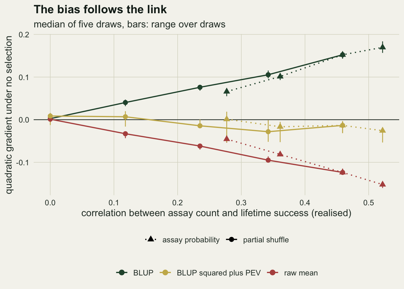
The standard error decides what gets reported
A point bias becomes a false claim only through a test. The table counts the share of replicate studies under no selection, in the design above, that reject a zero quadratic term at the five per cent level, first with the ordinary least squares standard error and then with the heteroscedasticity-consistent HC3 sandwich estimator (Long and Ervin 2000), at three study sizes.
n_grid <- c(300, 600)
size_res <- lapply(seq_along(n_grid), function(k) {
  s <- cell_summary(run_cell(n_grid[k], "none", "prob", 0.6, 0, "nb", n_sweep, 32900 + 100 * k))
  cbind(n_anim = n_grid[k], s)
})
size_tab <- rbind(cbind(n_anim = n_anim, scen_tab[scen_tab$cell == "null", -1]),
                  do.call(rbind, size_res))
size_tab <- size_tab[size_tab$arm %in% c("blup", "raw", "cal", "first"), ]
size_tab$mc_se <- sqrt(size_tab$rej_hc3 * (1 - size_tab$rej_hc3) / size_tab$kept)
print(size_tab[order(size_tab$arm, size_tab$n_anim),
               c("n_anim", "arm", "g_med", "rej_ols", "rej_hc3", "mc_se", "kept")],
      digits = 3, row.names = FALSE)
n_anim arm g_med rej_ols rej_hc3 mc_se kept
150 blup 1.52e-01 0.1995 0.0694 0.00360 4997
300 blup 1.43e-01 0.2793 0.1333 0.00621 3000
600 blup 1.46e-01 0.4587 0.2977 0.00835 3000
150 cal -1.33e-02 0.0947 0.0638 0.00346 4997
300 cal -1.69e-02 0.0967 0.0590 0.00430 3000
600 cal -9.16e-03 0.1010 0.0537 0.00411 3000
150 first 9.32e-03 0.0477 0.0627 0.00344 4964
300 first 5.82e-03 0.0460 0.0630 0.00444 2999
600 first 1.73e-05 0.0530 0.0577 0.00426 3000
150 raw -1.24e-01 0.0568 0.1997 0.00566 4997
300 raw -1.23e-01 0.1357 0.3363 0.00863 3000
600 raw -1.20e-01 0.3197 0.5220 0.00912 3000rv <- function(n, arm, col = "rej_hc3") size_tab[size_tab$n_anim == n & size_tab$arm == arm, col]
fixed_hc3 <- gv("null, three assays each", "blup", "rej_hc3")
fixed_ols <- gv("null, three assays each", "blup", "rej_ols")At 150 animals the ordinary standard error makes the two field analyses look far more different than their biases are. The BLUP gradient rejects in 0.200 of studies with the ordinary standard error and 0.069 with HC3; the raw-mean gradient rejects in 0.057 with the ordinary standard error and 0.200 with HC3. The two move in opposite directions because the residual variance of a count rises with its mean. The extreme BLUPs belong to long-lived animals with large and variable success, so the ordinary standard error of the squared term is too small; the extreme raw means belong to single-assay animals with small and uniform success, so it is too large, and it hides a bias of comparable size.
With HC3 both rates grow with study size, as a fixed bias against a shrinking standard error must, and the raw mean rejects more often at every size because its gradient is less noisy: at 150 animals its replicate standard deviation is 0.13 against 0.19 for the BLUP. As the study grows from 150 to 600 animals, the BLUP rejection rate rises from 0.069 to 0.133 and 0.298, the raw-mean rate from 0.200 to 0.336 and 0.522, while the calibrated square stays at 0.064, 0.059 and 0.054 and the first assay at 0.063, 0.063 and 0.058. Monte Carlo standard errors on these rates are at most 0.009. A false disruptive result at 150 animals is mostly a matter of the standard error; at 600 it is the bias itself. The calibrated square is not safe with the ordinary standard error either, rejecting in 0.095 to 0.101 of studies.
HC3 is itself a little liberal here. In the design with three assays each, where no analysis is biased, it rejects in 0.067 of studies at 150 animals against 0.049 for the ordinary standard error, which is the level to compare the repairs with. A bootstrap over animals, as the selection checks post recommends, is the slower alternative.
What to report
Report the distribution of assay counts and its correlation with fitness before any gradient. The correlation is the quantity the bias scales with, it costs one line of R, and a reader cannot recover it from a table of gradients. If every animal was assayed the same number of times, say so: the problem does not arise, and a standardised BLUP gradient is then the true gradient shrunk by the reliability, which can be reported alongside it.
Do not put standardised BLUPs or raw means into a quadratic regression when the counts vary with fate. In this design the two gave opposite signs with no selection present, and under real selection one erased it or reversed it while the other matched the truth only by cancellation. Neither answer is usable, and agreement between them would not mean much either.
For a test of whether any curvature exists, regress relative fitness on the BLUP and on the squared BLUP plus PEV, each divided by the among-individual variance, and use a heteroscedasticity-consistent standard error. That held a null rejection rate close to the HC3 baseline at every study size tried, with a small negative bias at the tightest links. For the size of the gradient, use a score of equal precision for every animal, such as the first assay, calibrated with the among-individual variance estimated as the variance of the first assays minus the within-animal variance of the repeat assays. Do not take the variances from the REML fit of all assays: when the behaviour affects survival, that estimate is pulled down and the gradient inflated. Report that the standard error leaves out the uncertainty in the variances, and say which of the two analyses the reported number comes from.
Do not add assay count as a covariate. It removes the artefact under no selection and removes most of the real selection when the behaviour affects survival, which is the case where assay count and fitness are linked for a biological reason.
Honest limits
The calibrations are plug-in. They treat the estimated variances and mean as known, so no standard error here carries their uncertainty, which is the part of the argument by Hadfield and colleagues that this post leaves alone. The moment variances remove the bias that selection on survival puts into the REML estimate, but not the cost of estimating: at 150 animals the first-assay gradient still sits about 6 per cent beyond its known-variance value under fecundity selection. The moment estimator also relies on every animal being assayed once before selection has sorted it. If animals enter the study at different ages, the first assays no longer share one distribution and the argument above for their variance fails. A model that fitted fitness and behaviour together would also need to represent how fitness depends on the assay count itself, or it would face the same weighting problem as the calibrated square.
Fitness is on the relative scale of the Lande-Arnold regression throughout, not on a latent scale. With negative binomial success and a lifespan that multiplies fecundity, a gradient on a log-link latent scale is a different quantity, and whether the oracle and the ranking of the repairs survive that change was not checked. The oracle itself is the best quadratic approximation to surfaces that are not quadratic, so a repair can differ from it slightly for that reason alone, most visibly under viability selection.
The strength of the link in real personality studies was not measured here. Many studies assay every animal a fixed number of times, where the problem vanishes, and many assay opportunistically at recapture, where the count follows survival. The sweeps show the bias growing roughly in proportion to the correlation between count and fitness, but no published value of that correlation was verified for this post, so the design above is an illustration of an opportunistic scheme and not an estimate for any species.
The first-assay repair assumes the first assay is comparable across animals. Here it is, because every animal is tested at the same age with the same variance. If the first test is also the first exposure to the arena and behaviour changes with experience, the first assay measures a different trait from the later ones. The obvious extension, keeping the first k assays of every animal that has k, conditions on having survived long enough to have them and brings the link straight back.
The behaviour is a single trait with a constant within-individual variance, and the only fixed effect is an intercept. Age trends in the behaviour, heterogeneous residual variance among animals, or a second correlated trait would each change the size of the biases; the sign argument from the table of expected squares survives all of them as long as precision rises with assay count. At 150 animals the replicate spread of every quadratic gradient here is wider than the gradient being estimated, which is the detection problem the nonlinear gradients post measures, and nothing about the repairs changes that.
References
Postma E 2006 Journal of Evolutionary Biology 19(2):309-320 (10.1111/j.1420-9101.2005.01007.x)
Hadfield JD, Wilson AJ, Garant D, Sheldon BC, Kruuk LEB 2010 American Naturalist 175(1):116-125 (10.1086/648604)
Houslay TM, Wilson AJ 2017 Behavioral Ecology 28(4):948-952 (10.1093/beheco/arx023)
Lande R, Arnold SJ 1983 Evolution 37(6):1210-1226 (10.1111/j.1558-5646.1983.tb00236.x)
Kingsolver JG, Hoekstra HE, Hoekstra JM, Berrigan D, Vignieri SN, Hill CE, Hoang A, Gibert P, Beerli P 2001 American Naturalist 157(3):245-261 (10.1086/319193)
Bell AM, Hankison SJ, Laskowski KL 2009 Animal Behaviour 77(4):771-783 (10.1016/j.anbehav.2008.12.022)
Long JS, Ervin LH 2000 The American Statistician 54(3):217-224 (10.1080/00031305.2000.10474549)