library(ggplot2)
library(patchwork)
library(nlme)

te_paper  <- "#f5f4ee"
te_ink    <- "#16241d"
te_body   <- "#2c3a31"
te_forest <- "#275139"
te_rust   <- "#b5534e"
te_gold   <- "#c9b458"
te_line   <- "#dad9ca"

theme_datasheet <- function() {
  theme_minimal(base_size = 12) +
    theme(plot.background  = element_rect(fill = te_paper, colour = NA),
          panel.background = element_rect(fill = te_paper, colour = NA),
          panel.grid.major = element_line(colour = te_line, linewidth = 0.3),
          panel.grid.minor = element_blank(),
          text             = element_text(colour = te_body),
          plot.title       = element_text(colour = te_ink, face = "bold"),
          plot.subtitle    = element_text(colour = te_body),
          axis.text        = element_text(colour = te_body))
}Per chick or per nest: informative cluster size
R
mixed models
nlme
clustered data
experimental design
simulation
ecology tutorial
When brood size tracks territory quality differently in fed and control nests, per-chick and per-nest effects can take opposite signs. Six estimators in R.
A food supplementation experiment on a nest box population: sixty territories get a feeder and sixty do not, and every chick is weighed at day twelve. The data frame has one row per chick, a column for the feeding treatment and a column for the nest. The obvious model regresses chick mass on treatment, and the obvious correction for the fact that chicks in one nest share parents and a territory is a random intercept for nest. Neither step asks the question that decides the answer: is the unit of the treatment effect a chick or a nest?
The two are different estimands whenever the number of chicks in a nest carries information about how heavy they are. That situation has a name, informative cluster size, and it is a published result rather than something this post found. Hoffman, Sen and Weinberg (2001) proposed within-cluster resampling for it, Williamson, Datta and Satten (2003) showed that a generalised estimating equation weighted by one over cluster size is asymptotically equivalent, and Seaman, Pavlou and Copas reviewed both the problem and its repairs in two 2014 papers. This post is a demonstration of those results on a brood-supplementation design, with every number computed below.
The closest post on the site is grouped summaries, which shows in its section on the mean of ratios that the pooled proportion and the mean of per-quadrat proportions are two correct answers to two different questions, and in the section after it that the pooled value is the quadrat mean weighted by quadrat total. That is the same identity as here, stated descriptively, with no model and no test. Put a treatment into the data and the two correct answers can take opposite signs, the per-chick one often comes back significant even with a standard error that respects the nests, the random intercept model sits between the two, and the repairs can be put in order by how often their intervals cover the effect.
Three other posts set the boundaries. GEE or a mixed model separates a marginal slope from a conditional one, but that gap comes from the curvature of a logit link, and its honest limits note that on an identity link the two coincide; everything here is on an identity link, and the two answers still differ by more than the effect. Within- and between-individual effects shows that an uncentred slope is a weighted average of two slopes and that centring the covariate separates them; that works because the covariate varies inside the cluster, and a feeding treatment is constant inside the nest, so there is nothing to centre. Pseudoreplication is about the standard error when nothing is biased. This post is about the estimate, and the draws below show how the two problems stack.
A feeding experiment where brood size carries territory quality
No published manipulation is modelled here. The meta-analytic evidence (Ruffino and colleagues 2014, 201 experiments) is that feeding advances laying and in many species enlarges the clutch, which is a different design; the honest limits at the end come back to it. The generator below is a stylised case, chosen because it isolates the weighting question.
Each territory has a quality, drawn once. Quality raises the mass of every chick raised there, and it also raises brood size, through a log-linear Poisson model with a coupling coefficient. The design question is what feeding does to that coupling. In the generator below it does one thing only: in fed territories brood size depends much less on quality, because food is no longer the constraint that ties the two together. The brood-size intercept is re-centred in each arm so that feeding does not change the mean brood size, and feeding enters chick mass only through its true effect of 0.25 g per nest. Nothing is confounded and there is no causal path from treatment to mass through brood size. Feeding makes every chick heavier; what it changes is which territories the chicks come from.
n_nest     <- 120    # territories, half fed
b_true     <- 0.25   # feeding effect on chick mass, grams, per nest
c_control  <- 0.9    # how strongly quality sets brood size without food
c_fed      <- 0.1    # the same coupling with a feeder
brood_mean <- 5      # mean of the Poisson part; brood size is 1 + Poisson
mass_base  <- 12     # grams at day twelve, average territory, no food
sd_chick   <- 0.8    # chick-to-chick scatter inside a nest, grams

make_broods <- function(n_nest, b = b_true, c_ctl = c_control, c_trt = c_fed,
                        sd_e = sd_chick) {
  fed     <- rep(0:1, each = n_nest / 2)
  quality <- rnorm(n_nest)
  coup    <- ifelse(fed == 1, c_trt, c_ctl)
  lam     <- exp(log(brood_mean) - coup^2 / 2 + coup * quality)  # mean 5 in both arms
  brood   <- 1L + rpois(n_nest, lam)
  mu      <- mass_base + b * fed + quality
  nest_id <- rep(seq_len(n_nest), brood)
  mass    <- mu[nest_id] + rnorm(sum(brood), 0, sd_e)
  list(chick = data.frame(mass = mass, fed = fed[nest_id],
                          nest = factor(nest_id), brood = brood[nest_id]),
       nests = data.frame(mass_bar = as.vector(tapply(mass, nest_id, mean)),
                          fed = fed, brood = brood, quality = quality))
}
One data set, and the four analyses a reader is most likely to run on it: ordinary least squares on chicks, the same regression with each chick weighted by one over its brood size, least squares on the 120 nest means, and a random intercept for nest fitted with nlme::lme.
set.seed(2403)
one <- make_broods(n_nest)
fit_chick <- lm(mass ~ fed, data = one$chick)
fit_w     <- lm(mass ~ fed, data = one$chick, weights = 1 / brood)
fit_nest  <- lm(mass_bar ~ fed, data = one$nests)
fit_ri    <- lme(mass ~ fed, random = ~ 1 | nest, data = one$chick)
row_of <- function(fit) summary(fit)$coefficients["fed", ]
one_tab <- rbind(per_chick = row_of(fit_chick)[c(1, 2, 4)],
                 weighted  = row_of(fit_w)[c(1, 2, 4)],
                 per_nest  = row_of(fit_nest)[c(1, 2, 4)],
                 random_int = summary(fit_ri)$tTable["fed", c(1, 2, 5)])
colnames(one_tab) <- c("estimate", "se", "p")
n_chicks_one <- nrow(one$chick)
round(one_tab, 4)
estimate se p
per_chick -0.7721 0.0923 0.0000
weighted -0.0239 0.0954 0.8022
per_nest -0.0239 0.2040 0.9069
random_int -0.1061 0.2009 0.5985The 749 chicks say that feeding changed mass by -0.772 g, with a p value of \(2.99 \times 10^{-16}\). The 120 nests say -0.024 g, p = 0.907: nothing at all, in a draw where the true per-nest effect is +0.25 g. That is the first data set drawn at the seed chosen before any analysis, and it is honest about the design, which has 120 nests and a standard error of 0.20 g for a quarter-gram effect; the next section counts how often the nest answer is positive. The weighted chick regression returns the per-nest estimate, -0.024 g, with a standard error of 0.095 against the nest regression’s 0.204. The random intercept model lands at -0.106 g, between the two.
arm_lab <- c("control", "fed")
nd <- one$nests; nd$arm <- factor(arm_lab[nd$fed + 1], levels = arm_lab)
p_couple <- ggplot(nd, aes(quality, brood, colour = arm)) +
  geom_point(size = 2, alpha = 0.8) +
  scale_colour_manual(values = c(te_gold, te_forest), name = NULL) +
  labs(x = "territory quality", y = "brood size",
       title = "Quality sets brood size", subtitle = "strongly without food, weakly with it") +
  theme_datasheet() + theme(legend.position = "bottom")

arm_means <- data.frame(
  arm = factor(rep(arm_lab, 2), levels = arm_lab),
  unit = factor(rep(c("per chick", "per nest"), each = 2), levels = c("per chick", "per nest")),
  mass = c(tapply(one$chick$mass, one$chick$fed, mean),
           tapply(one$nests$mass_bar, one$nests$fed, mean)))
p_means <- ggplot(arm_means, aes(arm, mass, colour = unit, group = unit)) +
  geom_line(linewidth = 1) + geom_point(size = 3) +
  scale_colour_manual(values = c(te_rust, te_ink), name = NULL) +
  labs(x = NULL, y = "mean chick mass (g)",
       title = "Two averages, one data set", subtitle = "large control broods lift the chick mean") +
  theme_datasheet() + theme(legend.position = "bottom")

p_couple + p_means + plot_annotation(theme = theme_datasheet())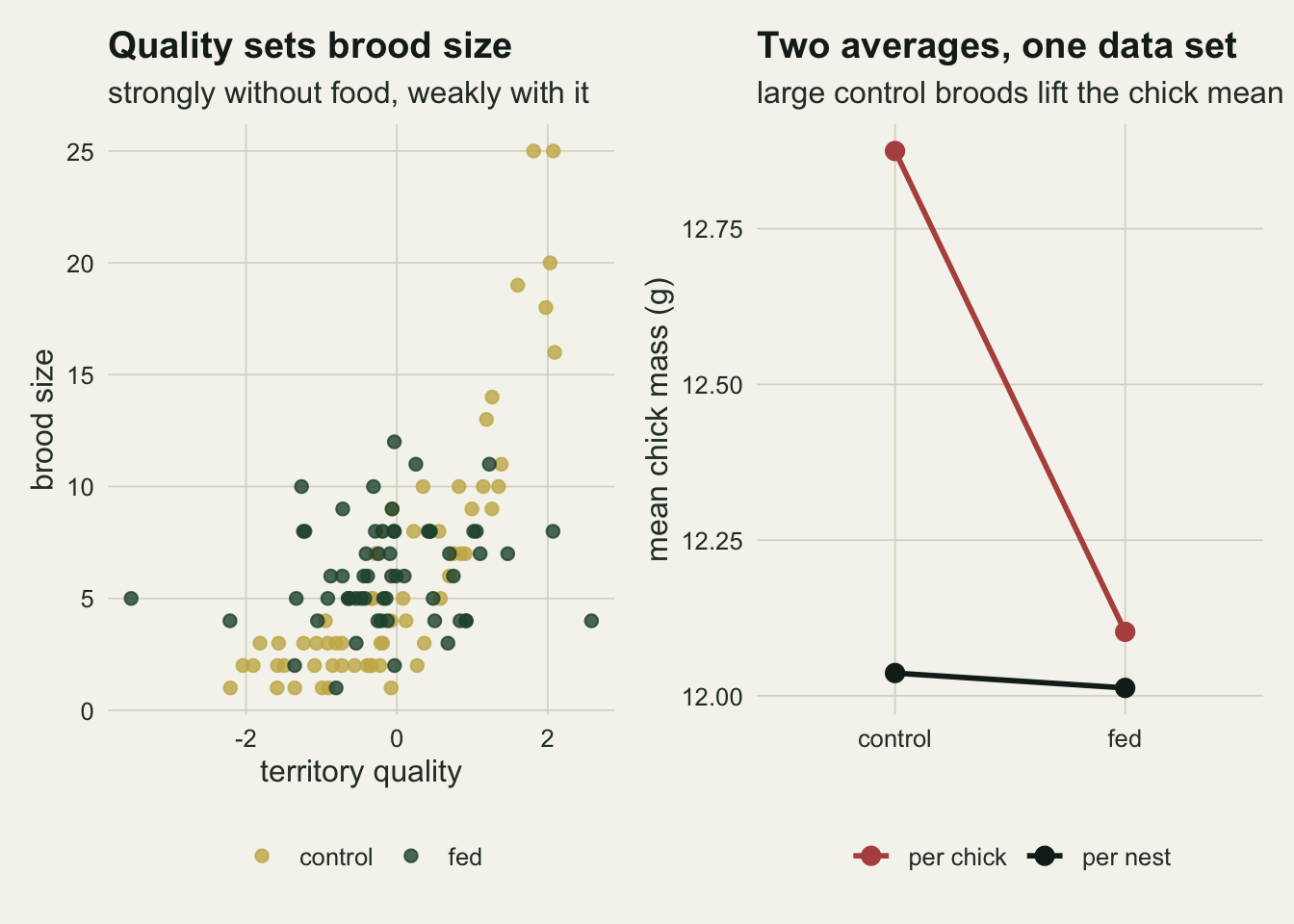
Two correct answers, derived
Neither estimate is wrong. The per-nest contrast estimates the effect of feeding on the average nest, which is 0.25 g by construction. The per-chick contrast estimates the effect on the average chick, and a nest enters that average with a weight equal to its brood size. The individual-weighted mean of the nest means differs from their plain mean by the covariance of brood size and nest mean divided by the mean brood size. In the control arm, where large broods sit in good territories, that covariance is large and the per-chick mean is pulled up; in the fed arm it is small. The two shifts do not cancel, and their difference is subtracted from the effect.
For this generator the shift has a closed form. Brood size is one plus a Poisson count with mean exp(a + c q), so its expectation is six, and the expectation of the Poisson mean times quality is c times five (for standard normal q, the Gaussian identity E[q exp(c q)] = c exp(c^2 / 2), a case of Stein’s lemma). The per-chick arm mean therefore sits 5c/6 g above the per-nest arm mean, and the per-chick contrast is 0.25 + 5(c_fed - c_control)/6.
chick_estimand <- function(c_ctl, c_trt, b = b_true) b + brood_mean * (c_trt - c_ctl) / (1 + brood_mean)
closed_chick <- chick_estimand(c_control, c_fed)
set.seed(9901)
big <- make_broods(40000)
big_chick <- unname(coef(lm(mass ~ fed, data = big$chick))["fed"])
big_nest  <- unname(coef(lm(mass_bar ~ fed, data = big$nests))["fed"])
brood_q <- sapply(split(big$nests$brood, big$nests$fed), quantile, probs = c(0.5, 0.95, 1))
brood_avg <- tapply(big$nests$brood, big$nests$fed, mean)
brood_cv  <- tapply(big$nests$brood, big$nests$fed, function(x) sd(x) / mean(x))
brood_cor <- sapply(split(big$nests, big$nests$fed), function(z) cor(z$brood, z$quality))
cv_poisson <- sqrt(brood_mean) / (1 + brood_mean)  # brood CV with no coupling at all
cv_small   <- 0.3    # an illustrative brood-size CV, below the Poisson floor
need_cor   <- b_true / (cv_small * 1)  # control correlation needed if fed nests have none
round(c(closed = closed_chick, big_chick = big_chick, big_nest = big_nest), 4)
closed big_chick big_nest
-0.4167 -0.4301 0.2504 brood_q 0 1
50% 4 6
95% 16 10
100% 134 18round(rbind(cv = brood_cv, cor = brood_cor, shift = brood_cv * brood_cor), 3) 0 1
cv 1.036 0.383
cor 0.737 0.212
shift 0.763 0.081With a pencil the per-chick estimand is -0.4167 g; a single draw of 40000 nests gives -0.4301 g per chick and +0.2504 g per nest. The size of the reversal is arithmetic, not a finding: once the two couplings are fixed, the gap between the estimands follows. The mean brood size in that large draw is 6.00 in control nests and 6.01 in fed ones, as designed, but the spread is not: the median control brood is 4 chicks, the 95th percentile 16 and the largest 134, while fed broods run to a maximum of 18. The coefficient of variation of brood size is 1.04 in control nests and 0.38 in fed ones; a brood of one plus a Poisson count with this mean, with no coupling at all, already has 0.37, and passerine clutches usually vary less than a Poisson count.
That spread is what the reversal runs on, and a bound shows how much. The shift in one arm is a covariance over a mean, so it equals the correlation between brood size and nest mean, times the coefficient of variation of brood size, times the standard deviation of the true nest means within the arm, which is 1 g here. In the large draw the correlation is 0.74 in control nests, so the control shift is 0.737 times 1.036 times 1, or 0.763 g, close to the 5c/6 = 0.75 above. With a coefficient of variation of 0.3 and the same 1 g spread among nests, no arm can shift by more than 0.3 g, so reversing a quarter-gram effect needs a correlation of at least 0.83 between brood size and nest mean in control nests and almost none in fed ones. The generator here sits far beyond what a nest box passerine shows, and the sweep further down includes a milder coupling for that reason.
What is not arithmetic is what a single experiment of 120 nests does with this, and which answer comes back significant.
Four hundred experiments, and the control
The same design is now run as 400 independent experiments, and again with the coupling set to 0.9 in both arms. The second set is the necessary control: brood size is then just as informative about quality, but equally so in both arms.
contrast_t <- function(y, g) {
  n1 <- sum(g); n0 <- length(g) - n1
  m1 <- sum(y * g) / n1; m0 <- sum(y * (1 - g)) / n0
  se <- sqrt(sum((y - ifelse(g == 1, m1, m0))^2) / (length(y) - 2) * (1 / n0 + 1 / n1))
  c(est = m1 - m0, se = se, p = 2 * pt(-abs((m1 - m0) / se), length(y) - 2))
}
cluster_p <- function(y, g, nest) {  # chick contrast, nest-clustered standard error
  n1 <- sum(g); n0 <- length(g) - n1
  m1 <- sum(y * g) / n1; m0 <- sum(y * (1 - g)) / n0
  s_nest <- rowsum(y - ifelse(g == 1, m1, m0), nest)  # per-nest residual sums
  g_nest <- rowsum(g, nest) > 0
  se <- sqrt(sum(s_nest[g_nest]^2) / n1^2 + sum(s_nest[!g_nest]^2) / n0^2)
  2 * pnorm(-abs((m1 - m0) / se))
}
two_contrasts <- function(d, mixed = FALSE) {
  a <- contrast_t(d$chick$mass, d$chick$fed); z <- contrast_t(d$nests$mass_bar, d$nests$fed)
  out <- c(chick = a[["est"]], p_chick = a[["p"]],
           p_chick_cl = cluster_p(d$chick$mass, d$chick$fed, d$chick$nest),
           nest = z[["est"]], p_nest = z[["p"]], max_ctl = max(d$nests$brood[d$nests$fed == 0]))
  if (mixed) {
    tt <- summary(lme(mass ~ fed, random = ~ 1 | nest, data = d$chick))$tTable["fed", ]
    out <- c(out, ri = tt[["Value"]], p_ri = tt[["p-value"]])
  }
  out
}
n_draw <- 400     # fixed before any rate was inspected
set.seed(5117)
diff_arm  <- t(replicate(n_draw, two_contrasts(make_broods(n_nest), mixed = TRUE)))
set.seed(5118)
equal_arm <- t(replicate(n_draw, two_contrasts(make_broods(n_nest, c_trt = c_control), mixed = TRUE)))
summ_arm <- function(z) c(
  disagree = mean(sign(z[, "chick"]) != sign(z[, "nest"])),
  chick_neg_sig = mean(z[, "chick"] < 0 & z[, "p_chick"] < 0.05),
  chick_neg_sig_cl = mean(z[, "chick"] < 0 & z[, "p_chick_cl"] < 0.05),
  ri_neg_sig = mean(z[, "ri"] < 0 & z[, "p_ri"] < 0.05), ri_neg = mean(z[, "ri"] < 0),
  nest_pos_sig = mean(z[, "nest"] > 0 & z[, "p_nest"] < 0.05),
  nest_pos_ns = mean(z[, "nest"] > 0 & z[, "p_nest"] >= 0.05),
  chick_mean = mean(z[, "chick"]), nest_mean = mean(z[, "nest"]),
  gap_mean = mean(z[, "chick"] - z[, "nest"]))
arm_tab <- rbind(differential = summ_arm(diff_arm), equal = summ_arm(equal_arm))
first10 <- sum(sign(diff_arm[1:10, "chick"]) != sign(diff_arm[1:10, "nest"]))
mcse_share <- function(p) sqrt(p * (1 - p) / n_draw)
max_ctl_q <- quantile(diff_arm[, "max_ctl"], c(0, 0.5, 1))
round(arm_tab, 3)
disagree chick_neg_sig chick_neg_sig_cl ri_neg_sig ri_neg
differential 0.820 0.725 0.312 0.005 0.185
equal 0.178 0.088 0.010 0.000 0.112
nest_pos_sig nest_pos_ns chick_mean nest_mean gap_mean
differential 0.272 0.630 -0.369 0.264 -0.633
equal 0.250 0.635 0.242 0.255 -0.013set.seed(5119)
chick_480 <- mean(replicate(n_draw, two_contrasts(make_broods(480))[["chick"]]))Under differential coupling the per-chick and per-nest contrasts disagree in sign in 82.0 per cent of the 400 experiments (Monte Carlo standard error 1.9 points), and in 6 of the first ten, which is how far a batch of ten experiments can wander from the rate. The per-nest contrast is positive and significant in 27.3 per cent of them, because 120 nests carry little power for a quarter of a gram, and positive but not significant in another 63.0 per cent.
How often the per-chick contrast reports a significant harmful effect depends on the standard error put on it. With chick-level least squares, which treats every chick as independent, it is 72.5 per cent of experiments, and most of that is pseudoreplication. With a nest-clustered standard error (built from the per-nest sums of chick residuals in each arm, with a normal reference as for the sandwich estimators further down) it is 31.2 per cent, and that part is the estimand shift alone: an apparently harmful effect of food on the average chick, which exists only because fed and control chicks come from different mixes of territories. The random intercept model, the obvious correction from the opening, reports significant harm in 0.5 per cent of experiments and a negative estimate at all in 18.5 per cent. Its damage is not a false verdict but the bias measured further down.
The per-chick contrast averages -0.369 g over the draws, short of the closed form -0.417. That is the finite-sample bias of a ratio: the per-chick arm mean divides one random sum by another, and with a long-tailed brood size it takes many nests to settle. The largest control brood in one experiment has a median of 27 chicks over the draws, and ranges from 12 to 149. With 480 nests the average is -0.402 g.
With equal coupling the two contrasts average +0.242 and +0.255 g, a mean gap of -0.013 g against -0.633 g under differential coupling. They still disagree in sign 17.8 per cent of the time, but that is noise around a small effect rather than a shift, since on average the two land in the same place. This is why the trap is invisible in most data sets. Informative cluster size alone moves both arms by the same amount and the contrast survives; what reverses it is cluster size that is informative by different amounts in the groups being compared. The equal arm also shows the other, older problem: the per-chick contrast is negative and significant in 8.8 per cent of draws even though its estimand is +0.25, because its standard error ignores the nests; with the nest-clustered standard error the share falls to 1.0 per cent. That part is pseudoreplication, and it stacks on top of the estimand problem.
draw_df <- rbind(data.frame(diff_arm[, c("chick", "nest")], design = "coupling differs between arms"),
                 data.frame(equal_arm[, c("chick", "nest")], design = "coupling equal in both arms"))
ggplot(draw_df, aes(nest, chick, colour = design)) +
  geom_hline(yintercept = 0, linetype = "dashed", colour = te_body, linewidth = 0.4) +
  geom_vline(xintercept = 0, linetype = "dashed", colour = te_body, linewidth = 0.4) +
  geom_abline(slope = 1, intercept = 0, linetype = "dotted", colour = te_ink, linewidth = 0.5) +
  geom_point(size = 1.4, alpha = 0.55) +
  scale_colour_manual(values = c(te_rust, te_forest), name = NULL) +
  labs(x = "per-nest effect of feeding (g)", y = "per-chick effect of feeding (g)",
       title = "Same experiments, two units",
       subtitle = "lower right: food helps the average nest and apparently harms the average chick") +
  theme_datasheet() + theme(legend.position = "bottom")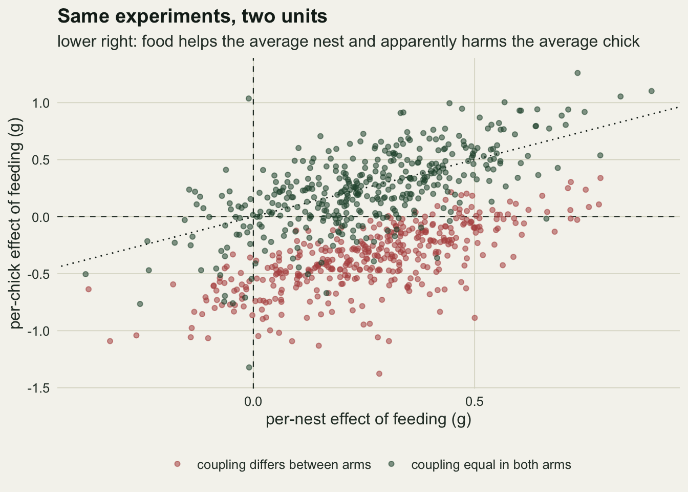
How wide the coupling gap has to be
The fed-arm coupling of 0.1 is an extreme choice, and the control coupling of 0.9 produces the long brood tail noted above. The sweep below keeps the per-nest effect at 0.25 g and walks the fed-arm coupling from zero up to the control value, for the main control coupling and for a milder one of 0.5.
n_sweep <- 200
sweep_grid <- rbind(data.frame(c_ctl = c_control, c_trt = seq(0, c_control, by = 0.1)),
                    data.frame(c_ctl = 0.5, c_trt = seq(0, 0.5, by = 0.1)))
set.seed(6240)
sweep_tab <- do.call(rbind, lapply(seq_len(nrow(sweep_grid)), function(i) {
  cc <- sweep_grid$c_ctl[i]; ct <- sweep_grid$c_trt[i]
  z <- t(replicate(n_sweep, two_contrasts(make_broods(n_nest, c_ctl = cc, c_trt = ct))))
  data.frame(c_ctl = cc, c_trt = ct, chick = mean(z[, "chick"]), nest = mean(z[, "nest"]),
             closed = chick_estimand(cc, ct), chick_sd = sd(z[, "chick"]),
             disagree = mean(sign(z[, "chick"]) != sign(z[, "nest"])),
             neg_sig = mean(z[, "chick"] < 0 & z[, "p_chick"] < 0.05),
             neg_sig_cl = mean(z[, "chick"] < 0 & z[, "p_chick_cl"] < 0.05))
}))
sweep_tab$control <- factor(sprintf("control nests %.1f", sweep_tab$c_ctl),
                            levels = sprintf("control nests %.1f", c(c_control, 0.5)))
cross_main <- c_control - b_true * (1 + brood_mean) / brood_mean
cross_mild <- 0.5 - b_true * (1 + brood_mean) / brood_mean
sw_at <- function(cc, ct, col) sweep_tab[[col]][abs(sweep_tab$c_ctl - cc) < 1e-9 & abs(sweep_tab$c_trt - ct) < 1e-9]
set.seed(6241)
mild_brood <- make_broods(40000, c_ctl = 0.5)$nests
mild_q <- quantile(mild_brood$brood[mild_brood$fed == 0], c(0.95, 1))
mild_cv <- sd(mild_brood$brood[mild_brood$fed == 0]) / mean(mild_brood$brood[mild_brood$fed == 0])
off_pts <- sweep_tab$c_trt < sweep_tab$c_ctl - 1e-9
n_up <- sum(sweep_tab$chick[off_pts] > sweep_tab$closed[off_pts])
sweep_gap <- max(abs(sweep_tab$chick - sweep_tab$closed))
sweep_mcse <- median(sweep_tab$chick_sd) / sqrt(n_sweep)
round(sweep_tab[, c("c_ctl", "c_trt", "chick", "closed", "disagree", "neg_sig", "neg_sig_cl")], 3)
c_ctl c_trt chick closed disagree neg_sig neg_sig_cl
1 0.9 0.0 -0.494 -0.500 0.855 0.880 0.510
2 0.9 0.1 -0.410 -0.417 0.860 0.770 0.365
3 0.9 0.2 -0.333 -0.333 0.785 0.720 0.275
4 0.9 0.3 -0.228 -0.250 0.690 0.565 0.130
5 0.9 0.4 -0.141 -0.167 0.515 0.465 0.070
6 0.9 0.5 -0.069 -0.083 0.475 0.330 0.055
7 0.9 0.6 0.035 0.000 0.345 0.210 0.025
8 0.9 0.7 0.132 0.083 0.220 0.175 0.015
9 0.9 0.8 0.151 0.167 0.250 0.125 0.005
10 0.9 0.9 0.232 0.250 0.215 0.105 0.015
11 0.5 0.0 -0.164 -0.167 0.645 0.455 0.110
12 0.5 0.1 -0.069 -0.083 0.515 0.275 0.040
13 0.5 0.2 0.029 0.000 0.390 0.135 0.005
14 0.5 0.3 0.094 0.083 0.240 0.065 0.020
15 0.5 0.4 0.170 0.167 0.140 0.075 0.005
16 0.5 0.5 0.235 0.250 0.095 0.035 0.005The per-chick estimand crosses zero where the coupling gap equals 0.25 times six fifths, that is at a fed-arm coupling of 0.6 when the control coupling is 0.9, and at 0.2 when it is 0.5. The simulated per-chick means follow the closed form to within 0.048 g at every point, and at 13 of the 14 points where the couplings differ they sit above it, towards the per-nest effect: that is the ratio bias described above, not noise (the Monte Carlo standard error is about 0.020 g per point). With the milder control coupling the control broods reach a 95th percentile of 13 and a maximum of 39 chicks, and the per-chick estimand turns negative only for a fed-arm coupling below 0.2: even at zero coupling the contrasts disagree in sign in 64 per cent of experiments, and the per-chick contrast is negative and significant with a nest-clustered standard error in 11 per cent (46 per cent with the chick-level one). At the main control coupling a fed-arm coupling of 0.3, a third of the control value, still gives 69 per cent disagreement, but significant harm with the clustered standard error in only 13 per cent. The rates carry a Monte Carlo standard error of at most 3.5 points each.
p_est <- ggplot(sweep_tab, aes(c_trt, chick, colour = control)) +
  geom_hline(yintercept = b_true, linetype = "dashed", colour = te_ink, linewidth = 0.5) +
  geom_hline(yintercept = 0, colour = te_body, linewidth = 0.3) +
  geom_line(aes(y = closed), linewidth = 0.9) +
  geom_point(size = 2.2, shape = 21, fill = te_paper, stroke = 0.9) +
  scale_colour_manual(values = c(te_rust, te_gold), name = NULL) +
  labs(x = "brood size coupling in fed nests", y = "per-chick effect (g)",
       title = "The per-chick estimand", subtitle = "dashed: the per-nest effect, 0.25 g") +
  theme_datasheet() + theme(legend.position = "bottom")
p_dis <- ggplot(sweep_tab, aes(c_trt, disagree, colour = control)) +
  geom_line(linewidth = 0.9) + geom_point(size = 2.2) +
  scale_colour_manual(values = c(te_rust, te_gold), name = NULL, guide = "none") +
  scale_y_continuous(limits = c(0, 1)) +
  labs(x = "brood size coupling in fed nests", y = "share of experiments",
       title = "Sign disagreement", subtitle = "per chick against per nest") +
  theme_datasheet() + theme(legend.position = "bottom")
p_est + p_dis + plot_layout(guides = "collect") +
  plot_annotation(theme = theme_datasheet()) & theme(legend.position = "bottom")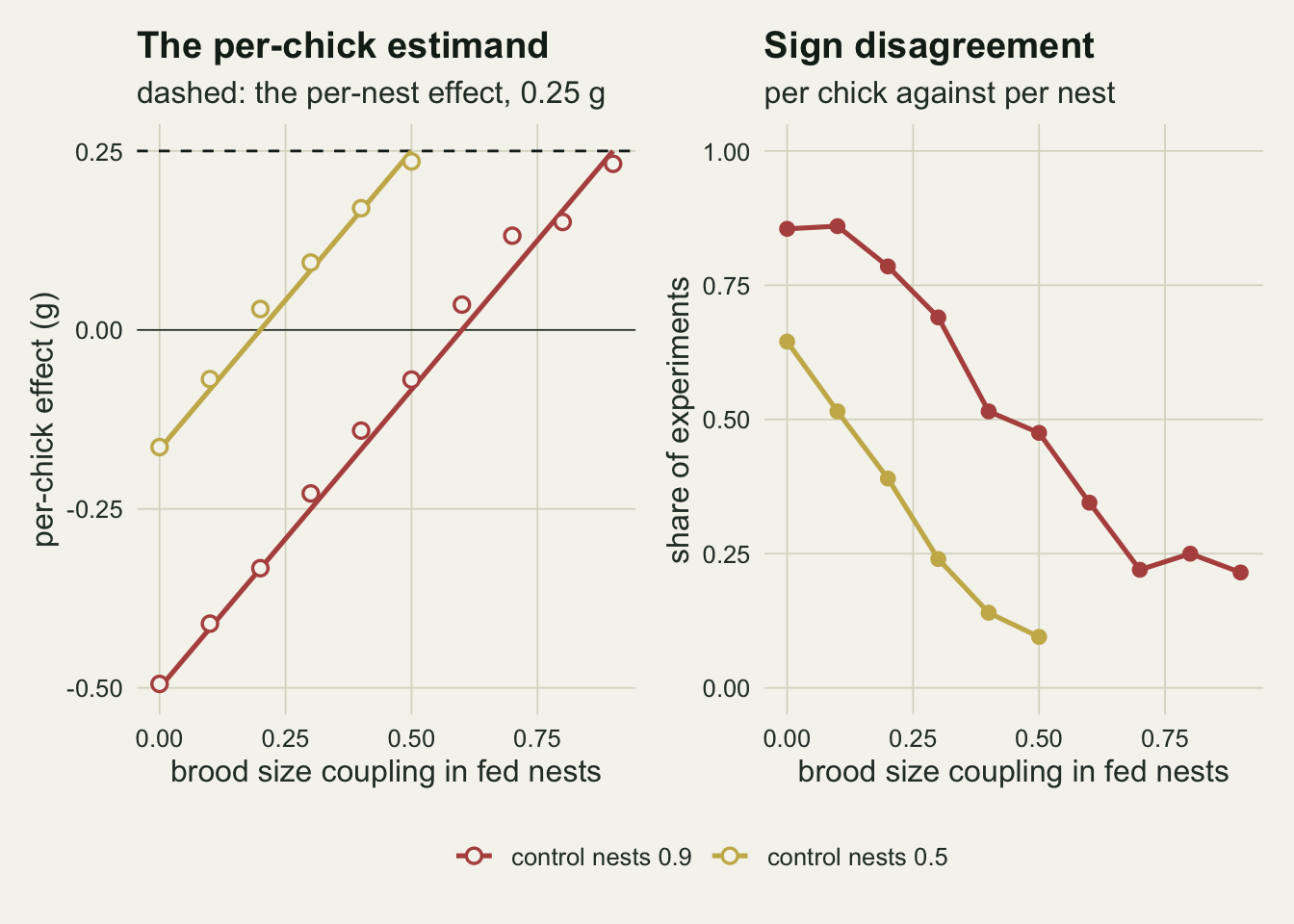
The weight is the nest-mean regression
Weighting each chick by one over its brood size is the usual first repair, and on the data set above it returned the per-nest estimate exactly. That is not a coincidence of this data set. With a covariate that is constant within the nest, the weighted least squares criterion sums, over nests, one over the brood size times the sum of squared chick residuals, and the normal equations collapse to those of an unweighted regression on the nest means. The point estimate is identical, not close. The standard error is not, because lm believes it has 749 observations with variances proportional to brood size.
Williamson, Datta and Satten’s cluster-weighted estimating equation is the same weighted estimate with a sandwich variance that sums the score over nests instead of chicks. Hoffman, Sen and Weinberg’s within-cluster resampling draws one chick per nest, fits the ordinary regression, repeats that many times and averages; its variance is the mean of the within-resample variances minus the variance of the resampled estimates. Both are written out below in base R.
cluster_se <- function(fit, cluster) {
  X <- model.matrix(fit); w <- weights(fit); e <- resid(fit)
  bread <- solve(crossprod(X, X * w))
  score <- rowsum(X * (w * e), cluster)
  sqrt((bread %*% crossprod(score) %*% bread)[2, 2])
}
wcr_fit <- function(d, n_resample) {
  g <- d$nests$fed; n_g <- length(g)
  first <- cumsum(c(0, d$nests$brood))[seq_len(n_g)]
  pick <- first + 1 + floor(matrix(runif(n_resample * n_g), nrow = n_g) * d$nests$brood)
  yq <- matrix(d$chick$mass[pick], nrow = n_g)
  m1 <- colMeans(yq[g == 1, , drop = FALSE]); m0 <- colMeans(yq[g == 0, , drop = FALSE])
  fitted_q <- outer(g, m1) + outer(1 - g, m0)
  var_q <- colSums((yq - fitted_q)^2) / (n_g - 2) * (1 / sum(g) + 1 / sum(1 - g))
  est_q <- m1 - m0
  c(est = mean(est_q), se = sqrt(mean(var_q) - var(est_q)))
}
r_nest <- resid(fit_nest); g1 <- one$nests$fed == 1
hc0_nest <- sqrt(sum(r_nest[g1]^2) / sum(g1)^2 + sum(r_nest[!g1]^2) / sum(!g1)^2)
set.seed(7730)
wcr_one <- wcr_fit(one, 4000)
id_tab <- rbind(
  weighted_lm = c(coef(fit_w)[["fed"]], row_of(fit_w)[["Std. Error"]]),
  nest_means  = c(coef(fit_nest)[["fed"]], row_of(fit_nest)[["Std. Error"]]),
  cluster_weighted_gee = c(coef(fit_w)[["fed"]], cluster_se(fit_w, one$chick$nest)),
  within_cluster_resampling = wcr_one)
colnames(id_tab) <- c("estimate", "se")
id_gap <- abs(coef(fit_w)[["fed"]] - coef(fit_nest)[["fed"]])
sand_gap <- abs(cluster_se(fit_w, one$chick$nest) - hc0_nest)
round(id_tab, 4)
estimate se
weighted_lm -0.0239 0.0954
nest_means -0.0239 0.2040
cluster_weighted_gee -0.0239 0.2023
within_cluster_resampling -0.0228 0.2039The weighted and nest-mean estimates agree to within floating-point rounding. The cluster-weighted sandwich standard error, 0.2023, is the heteroscedasticity-consistent standard error of the nest-mean regression, again equal to within floating-point rounding: with a nest-level treatment, the score of each nest is its nest-mean residual, so the sandwich is built from 120 residuals, one per nest. Within-cluster resampling with 4000 draws gives -0.0228 g with a standard error of 0.2039, the nest-mean answer up to resampling noise, since the average of a randomly chosen chick from each nest has the nest mean as its expectation.
So for a treatment applied to whole nests, the two named repairs and the one-over-size weight are all the nest-mean regression in different clothes. What separates them is which count of observations the standard error thinks it has.
Six estimators ranked by coverage
Coverage of the per-nest effect, 0.25 g, which is exact by construction and needs no reference draw. Each method uses its own software’s interval: t intervals on the residual degrees of freedom for the three lm fits, the lme t interval on its 118 denominator degrees of freedom, and normal intervals for the sandwich and the resampling estimator, as their authors define them.
n_rep <- 1000    # fixed before any coverage was inspected
n_wcr <- 100     # resamples per data set for within-cluster resampling
fit_six <- function(d) {
  f_chick <- lm(mass ~ fed, data = d$chick)
  f_w     <- lm(mass ~ fed, data = d$chick, weights = 1 / brood)
  f_nest  <- lm(mass_bar ~ fed, data = d$nests)
  f_ri    <- lme(mass ~ fed, random = ~ 1 | nest, data = d$chick)
  crit_c  <- qt(0.975, df.residual(f_chick)); crit_n <- qt(0.975, df.residual(f_nest))
  tt <- summary(f_ri)$tTable["fed", ]
  est <- c(coef(f_chick)[["fed"]], coef(f_w)[["fed"]], coef(f_nest)[["fed"]], tt[["Value"]],
           coef(f_w)[["fed"]], NA)
  half <- c(crit_c * row_of(f_chick)[["Std. Error"]], crit_c * row_of(f_w)[["Std. Error"]],
            crit_n * row_of(f_nest)[["Std. Error"]], qt(0.975, tt[["DF"]]) * tt[["Std.Error"]],
            qnorm(0.975) * cluster_se(f_w, d$chick$nest), NA)
  wc <- wcr_fit(d, n_wcr); est[6] <- wc[["est"]]; half[6] <- qnorm(0.975) * wc[["se"]]
  c(est, half)
}
est_lev <- c("chick OLS", "1/m-weighted OLS", "nest-mean OLS", "random intercept",
             "cluster-weighted GEE", "within-cluster resampling")
set.seed(8802)
cov_raw <- replicate(n_rep, fit_six(make_broods(n_nest)))
est_m <- cov_raw[1:6, ]; half_m <- cov_raw[7:12, ]
cov_tab <- data.frame(estimator = factor(est_lev, levels = est_lev),
                      bias = rowMeans(est_m) - b_true,
                      sd = apply(est_m, 1, sd),
                      coverage = rowMeans(abs(est_m - b_true) <= half_m),
                      width = rowMeans(2 * half_m))
cov_tab$mcse <- sqrt(cov_tab$coverage * (1 - cov_tab$coverage) / n_rep)
max_w_nest <- max(abs(est_m[2, ] - est_m[3, ]))
cv <- setNames(cov_tab$coverage, est_lev); bs <- setNames(cov_tab$bias, est_lev)
cov_tab[, -1] <- round(cov_tab[, -1], 3); cov_tab
estimator bias sd coverage width mcse
1 chick OLS -0.630 0.269 0.045 0.376 0.007
2 1/m-weighted OLS 0.004 0.190 0.671 0.373 0.015
3 nest-mean OLS 0.004 0.190 0.956 0.778 0.006
4 random intercept -0.080 0.188 0.929 0.767 0.008
5 cluster-weighted GEE 0.004 0.190 0.952 0.763 0.007
6 within-cluster resampling 0.004 0.190 0.952 0.768 0.007Over 1000 experiments the weighted and nest-mean estimates never differ by more than floating-point rounding, and they share a bias of +0.004 g. Their coverages are 0.671 and 0.956. Same numbers, two intervals, and only one of them honest.
The ranking is the result to carry away: the chick regression covers the per-nest effect almost never, the weighted chick regression covers it about two times in three, and every analysis that counts nests rather than chicks sits at or near the nominal 95 per cent. The cluster-weighted estimating equation reaches 0.952 and within-cluster resampling 0.952, which is the nest-mean interval with a normal critical value and 120 clusters. The Monte Carlo standard error near 0.95 is 0.007.
The random intercept model is the uncomfortable line. Its interval covers 0.929 of the time, 3.0 Monte Carlo standard errors short of nominal but not so short that anyone would notice in one study, and nothing in its output looks wrong, yet it is biased by -0.080 g, 32 per cent of the true effect. It weights each nest by one over the variance of its mean; that variance shrinks as the brood grows, so large broods count for more than one nest each, though far less than they do in the chick regression. The interval is wide enough to hide that shift at this sample size; a larger study would not be so lucky.
cov_plot <- data.frame(estimator = factor(est_lev, levels = rev(est_lev)),
                       coverage = cv, mcse = sqrt(cv * (1 - cv) / n_rep), bias = bs,
                       family = c("chick", "chick", "nest", "mixed", "nest", "nest"))
p_cov <- ggplot(cov_plot, aes(coverage, estimator, colour = family)) +
  geom_vline(xintercept = 0.95, linetype = "dashed", colour = te_body, linewidth = 0.5) +
  geom_errorbar(aes(xmin = coverage - 2 * mcse, xmax = coverage + 2 * mcse),
                orientation = "y", width = 0.3, linewidth = 0.5) +
  geom_point(size = 3) +
  scale_colour_manual(values = c(chick = te_rust, mixed = te_gold, nest = te_forest), guide = "none") +
  scale_x_continuous(limits = c(0, 1)) +
  labs(x = "coverage of the per-nest effect", y = NULL, title = "Coverage",
       subtitle = "dashed: nominal 0.95") +
  theme_datasheet()
p_bias <- ggplot(cov_plot, aes(bias, estimator, colour = family)) +
  geom_vline(xintercept = 0, colour = te_body, linewidth = 0.4) +
  geom_point(size = 3) +
  scale_colour_manual(values = c(chick = te_rust, mixed = te_gold, nest = te_forest), guide = "none") +
  labs(x = "bias (g)", y = NULL, title = "Bias", subtitle = "true per-nest effect 0.25 g") +
  theme_datasheet() + theme(axis.text.y = element_blank())
p_cov + p_bias + plot_layout(widths = c(1.4, 1)) + plot_annotation(theme = theme_datasheet())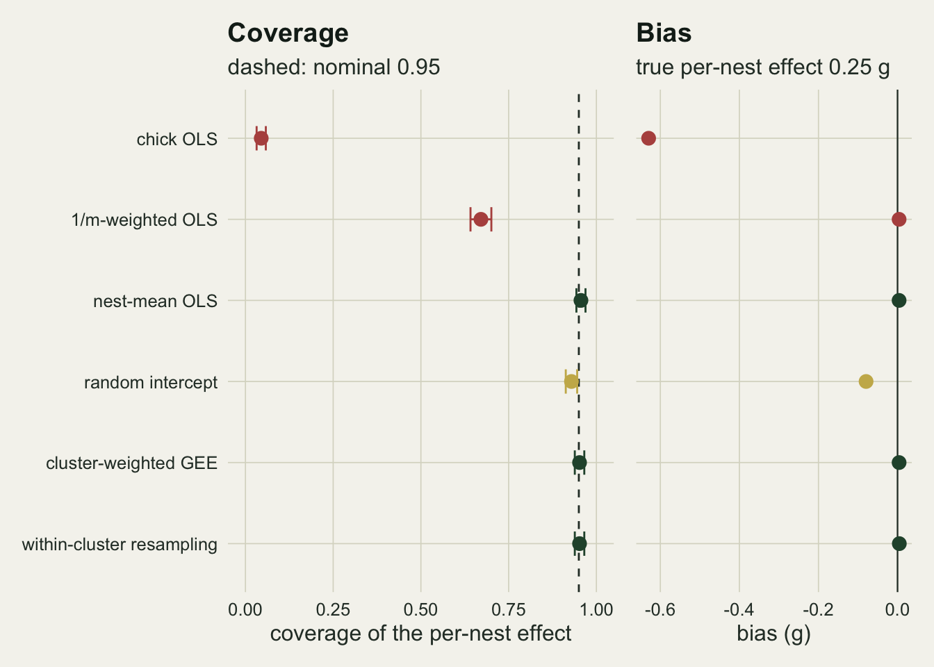
Where the random intercept lands
The random intercept estimate is a weighted average of nest means with weights one over the among-nest variance plus the within-nest variance divided by brood size. When the intraclass correlation is high, those weights are nearly equal and the model is the nest-mean regression; when it is low, they are nearly proportional to brood size and the model is the chick regression. The sweep changes the within-nest scatter and leaves everything else alone, so the intraclass correlation is one over one plus that variance.
sd_grid <- c(0.3, 0.8, 1.5, 3, 6)
n_icc <- 300
set.seed(9315)
icc_tab <- do.call(rbind, lapply(sd_grid, function(s) {
  z <- replicate(n_icc, {
    d <- make_broods(n_nest, sd_e = s)
    f_chick <- lm(mass ~ fed, data = d$chick)
    f_w <- lm(mass ~ fed, data = d$chick, weights = 1 / brood)
    f_nest <- lm(mass_bar ~ fed, data = d$nests)
    tt <- summary(lme(mass ~ fed, random = ~ 1 | nest, data = d$chick))$tTable["fed", ]
    cr <- qt(0.975, df.residual(f_chick))
    c(coef(f_chick)[["fed"]], cr * row_of(f_chick)[["Std. Error"]],
      coef(f_w)[["fed"]], cr * row_of(f_w)[["Std. Error"]],
      coef(f_nest)[["fed"]], qt(0.975, df.residual(f_nest)) * row_of(f_nest)[["Std. Error"]],
      tt[["Value"]], qt(0.975, tt[["DF"]]) * tt[["Std.Error"]])
  })
  hit <- function(k) abs(z[k, ] - b_true) <= z[k + 1, ]
  covr <- function(k) mean(hit(k))
  d_rw <- hit(7) - hit(3)  # random intercept minus 1/m weight, paired per experiment
  data.frame(sd_e = s, icc = 1 / (1 + s^2),
             position = (mean(z[7, ]) - mean(z[5, ])) / (mean(z[1, ]) - mean(z[5, ])),
             ri_bias = mean(z[7, ]) - b_true,
             cov_chick = covr(1), cov_w = covr(3), cov_nest = covr(5), cov_ri = covr(7),
             ri_minus_w = mean(d_rw), se_rw = sd(d_rw) / sqrt(n_icc))
}))
round(icc_tab, 3)
sd_e icc position ri_bias cov_chick cov_w cov_nest cov_ri ri_minus_w se_rw
1 0.3 0.917 0.023 -0.018 0.023 0.610 0.957 0.957 0.347 0.028
2 0.8 0.610 0.129 -0.084 0.050 0.637 0.947 0.913 0.277 0.026
3 1.5 0.308 0.306 -0.196 0.087 0.770 0.963 0.867 0.097 0.022
4 3.0 0.100 0.535 -0.353 0.297 0.813 0.940 0.760 -0.053 0.027
5 6.0 0.027 0.776 -0.485 0.737 0.873 0.947 0.830 -0.043 0.023ic <- function(s, col) icc_tab[[col]][icc_tab$sd_e == s]
worse_than_w <- icc_tab$icc[icc_tab$cov_ri < icc_tab$cov_w]
ri_worst <- any(icc_tab$cov_ri < pmin(icc_tab$cov_chick, icc_tab$cov_w))The position of the random intercept estimate on the axis from the nest regression (zero) to the chick regression (one) rises from 0.02 at an intraclass correlation of 0.92 to 0.13 at 0.61, the main design, and 0.78 at 0.027. Its bias goes from -0.018 to -0.485 g along the same path. So the bias is governed by the intraclass correlation together with the brood-size distribution and the coupling gap, which fix where the two ends of the axis lie; the correlation, through the weights it sets for each brood size, decides where between them the model sits.
Coverage follows. At the highest correlation the mixed model covers 0.957; at the lowest, 0.830, against 0.873 for the weighted chick regression and 0.737 for the plain chick regression. Across the whole sweep the mixed model stays above the plain chick regression, so it never becomes the worst of the four, but at intraclass correlations of 0.10 and below it covers less often than the one-over-size weighted chick regression, whose standard error is itself wrong; its lowest coverage, 0.760, is at 0.10. The two gaps behind that crossover are small, -0.053 and -0.043 in coverage, about 2.0 and 1.9 paired Monte Carlo standard errors, so the crossover is suggestive rather than settled. Coverage at the lowest correlation recovers a little, as every interval widens with the within-nest scatter. Each coverage here rests on 300 experiments, a Monte Carlo standard error of up to 0.029.
p_pos <- ggplot(icc_tab, aes(icc, position)) +
  geom_line(colour = te_gold, linewidth = 0.9) + geom_point(colour = te_gold, size = 2.4) +
  scale_x_log10() + scale_y_continuous(limits = c(0, 1)) +
  labs(x = "intraclass correlation (log scale)", y = "0 = per nest, 1 = per chick",
       title = "The mixed model drifts", subtitle = "towards the chick answer as ICC falls") +
  theme_datasheet()
cov_long <- data.frame(icc = rep(icc_tab$icc, 4),
  estimator = factor(rep(c("chick OLS", "1/m-weighted OLS", "nest-mean OLS", "random intercept"),
                         each = nrow(icc_tab)),
                     levels = c("chick OLS", "1/m-weighted OLS", "nest-mean OLS", "random intercept")),
  coverage = c(icc_tab$cov_chick, icc_tab$cov_w, icc_tab$cov_nest, icc_tab$cov_ri))
p_icc_cov <- ggplot(cov_long, aes(icc, coverage, colour = estimator, linetype = estimator)) +
  geom_hline(yintercept = 0.95, linetype = "dashed", colour = te_body, linewidth = 0.5) +
  geom_line(linewidth = 0.9) + geom_point(size = 2.2) +
  scale_x_log10() + scale_y_continuous(limits = c(0, 1)) +
  scale_colour_manual(values = c(te_rust, te_ink, te_forest, te_gold), name = NULL) +
  scale_linetype_manual(values = c("solid", "dotted", "solid", "solid"), name = NULL) +
  guides(colour = guide_legend(nrow = 2), linetype = guide_legend(nrow = 2)) +
  labs(x = "intraclass correlation (log scale)", y = "coverage", title = "Coverage by ICC",
       subtitle = "dashed: nominal 0.95") +
  theme_datasheet() + theme(legend.position = "bottom")
p_pos + p_icc_cov + plot_annotation(theme = theme_datasheet())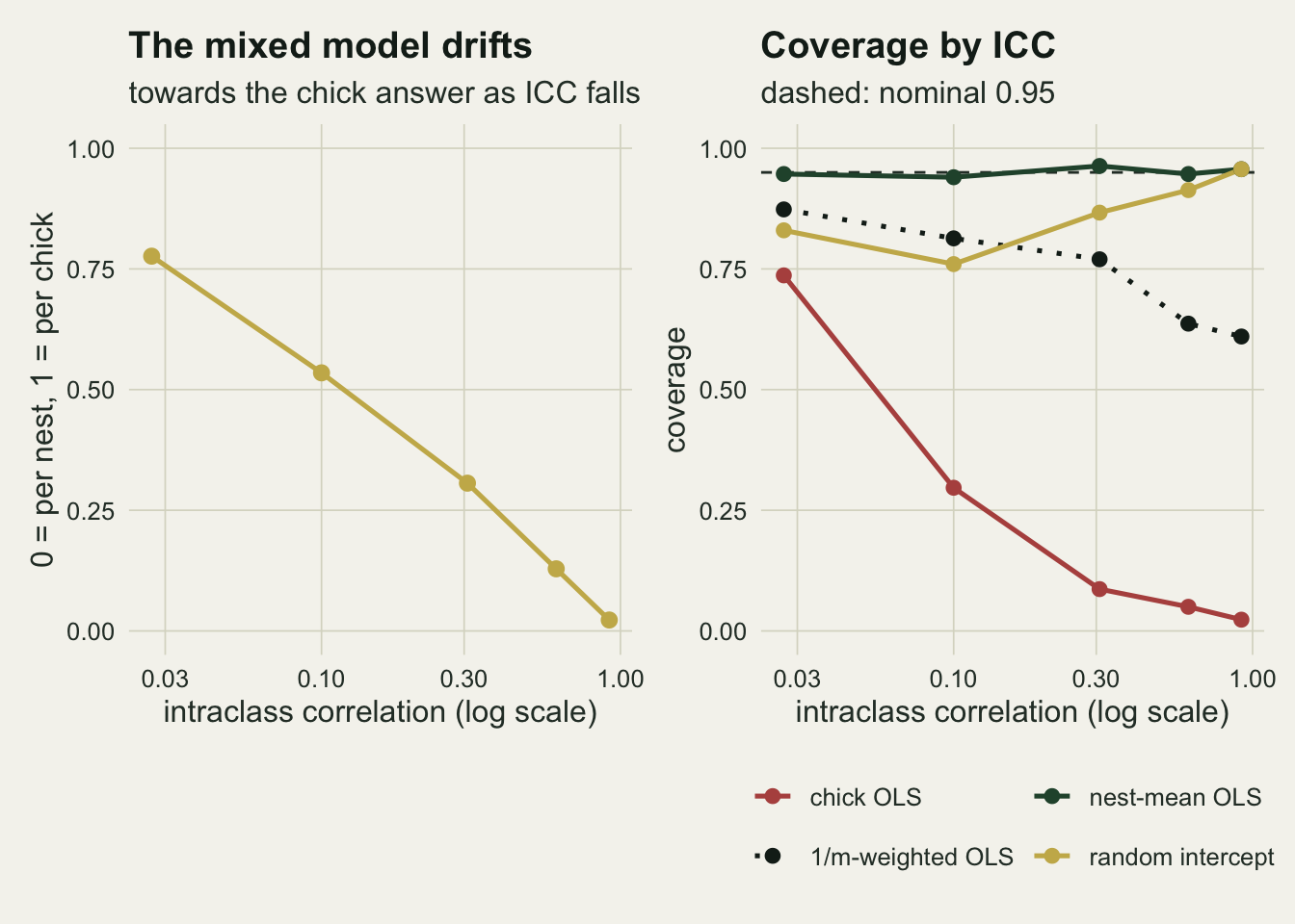
What to report
Say which unit the treatment effect is for before giving it. A feeding effect per nest and a feeding effect per chick are both legitimate, and they answer different management questions: whether putting out feeders improves the average territory, and whether the average fledgling in the population is heavier. A paper that reports one while describing the other has made the error the grouped-summaries post describes, now with a p value attached.
Report the cluster-size distribution in each arm, not only its mean. Here the means were equal by design and the problem sat entirely in how brood size covaried with quality. The direct check needs no quality proxy: plot nest-mean mass against brood size in each arm. Within an arm, the per-chick mean minus the per-nest mean is exactly the covariance of brood size and nest mean divided by the mean brood size, so the two contrasts differ by exactly the difference of that quantity between the arms.
arm_check <- sapply(split(one$nests, one$nests$fed), function(z) {
  cov_nm <- mean((z$brood - mean(z$brood)) * (z$mass_bar - mean(z$mass_bar)))
  c(cov_over_mean = cov_nm / mean(z$brood),
    chick_minus_nest = sum(z$brood * z$mass_bar) / sum(z$brood) - mean(z$mass_bar))
})
colnames(arm_check) <- c("control", "fed")
contrast_gap <- one_tab["per_chick", "estimate"] - one_tab["per_nest", "estimate"]
round(arm_check, 4)
control fed
cov_over_mean 0.8383 0.0901
chick_minus_nest 0.8383 0.0901In the data set from the top, the per-chick mean exceeds the per-nest mean by 0.8383 g in control nests and by 0.0901 g in fed nests, and the covariance over the mean brood size reproduces both. The difference of the two, -0.7482 g, is the gap between the per-chick and per-nest contrasts, -0.7482 g.
If the question is per nest and the treatment is applied per nest, the regression on nest means is the analysis. It has the right estimand and no fitting algorithm, its standard error is right when the arms are balanced (otherwise use the heteroscedasticity-consistent standard error, which is the cluster-weighted sandwich), and the cluster-weighted and resampling estimators reduce to it. Keep the chick rows for questions that vary within the nest, such as hatching order or sex.
If a random intercept model is used, report its estimate beside the nest-mean one. When the two differ by a noticeable fraction of the effect, cluster size is informative, and the mixed model is weighting nests by a rule set by the variance components rather than by the question.
Honest limits
As said where the generator is introduced, no named manipulation is modelled. Food supplementation in birds has variable effects that are mostly positive, and in many species it advances laying and enlarges the clutch (Ruffino and colleagues 2014 pool 201 experiments and find clutch-size responses strongest in food-caching species). A treatment that raises brood size in all territories is a different design: feeding then causes lighter chicks through a real path, and the per-chick contrast is a legitimate total effect rather than a weighting artefact. The decoupling assumed here, where food loosens the link between quality and brood size without changing its mean, is one mechanism an avian ecologist might defend for a species whose brood size is food-limited only in poor territories, and the post makes no claim that it is common: no study cited here documents it.
The control arm’s brood-size spread is far beyond a passerine’s: a coefficient of variation of 1.04, against 0.37 for a Poisson brood with no coupling at all. The milder coupling in the sweep cuts it to 0.58, still above the Poisson value, and there the reversal requires a fed-arm coupling below 0.2 and produces a significant harmful per-chick effect with a nest-clustered standard error in at most 11 per cent of experiments (46 per cent with the chick-level one). The post’s headline rates belong to the stronger design, and the bound in the derivation says that with a brood-size coefficient of variation of 0.3, reversing a quarter-gram effect needs a correlation of at least 0.83 between brood size and nest mean in control nests and almost none in fed ones.
Mass depends on quality through the nest mean only. If chick mass also fell with brood size inside a territory, through competition among siblings, the per-chick and per-nest estimands would differ even with equal coupling, and that difference would be part of the biology rather than a weighting choice.
The treatment is constant within the nest throughout. That is what makes the weighted, cluster-weighted and resampling estimators collapse onto the nest-mean regression, and the collapse does not depend on the link: with a nest-level treatment the weighted and cluster-weighted estimators reduce exactly to an unweighted analysis of nest means under any link (on a logit link, an unweighted quasi-binomial GLM on nest proportions), and within-cluster resampling does so as the number of nests grows. Williamson, Datta and Satten’s estimator and Hoffman, Sen and Weinberg’s resampling earn their keep when a covariate varies within the cluster, and that is not tested here. What the sandwich adds for a nest-level treatment is a standard error that survives unequal variances of the nest means, which balanced arms of 60 hide; with unbalanced arms whose brood-size distributions differ, the classical nest-mean standard error is no longer right, and the heteroscedasticity-consistent one is. Seaman, Pavlou and Copas (2014, Biometrics) also separate inference about all cluster members from inference about the observed ones, which matters when chicks die before weighing; every chick here is weighed.
Sample sizes are one design, 120 nests. The ratio bias of the per-chick estimate, the random intercept’s position, and the coverage gaps all depend on the number of nests, and a study with a few hundred nests would see a larger share of the mixed model’s bias show up as undercoverage.
References
Hoffman EB, Sen PK, Weinberg CR 2001 Biometrika 88(4):1121-1134 (10.1093/biomet/88.4.1121)
Williamson JM, Datta S, Satten GA 2003 Biometrics 59(1):36-42 (10.1111/1541-0420.00005)
Seaman SR, Pavlou M, Copas AJ 2014 Statistics in Medicine 33(30):5371-5387 (10.1002/sim.6277)
Seaman SR, Pavlou M, Copas AJ 2014 Biometrics 70(2):449-456 (10.1111/biom.12151)
Ruffino L, Salo P, Koivisto E, Banks PB, Korpimaki E 2014 Frontiers in Zoology 11:80 (10.1186/s12983-014-0080-y)