---
title: "GEE or a mixed model? Marginal and conditional"
description: "A GEE estimates the population-averaged effect and a GLMM the site-specific one. On a logit link they differ by a predictable factor; on a log link they do not."
date: "2026-08-12 14:00"
date-modified: "2026-10-01"
categories: [R, mixed models, GLM, lme4, ecology tutorial]
image: thumbnail.png
image-alt: "Logistic curves for many individual sites, a flatter dashed curve for their average, and a marginal model fit lying on top of the average."
---
*Corrected 1 October 2026: the missing-data paragraph illustrated the condition under which a mixed model stays valid with the weather and the effort at earlier visits, which are covariates and leave a GEE no worse off; it now uses detections at earlier visits, the kind of dependence that separates the two.*
Two ecologists analyse the same nested data set. One fits a mixed model with a random intercept for site, the other fits a generalised estimating equation with site as the cluster. Both are correct, both report a slope, and the two slopes are different. Not slightly different: on a logit link the difference is a factor that can be predicted, approximately, in advance, and it grows with how much the sites differ from one another.
Neither model is wrong. They are estimating different quantities, and the choice between them is a choice about which quantity the question is about.
## The two questions
A mixed model puts a random intercept on each site and estimates the slope holding that intercept fixed. Its answer is: if this site's conditions improve by one unit, how do the odds change at that site. That is a conditional, or subject-specific, effect.
A GEE models the mean of the response as a function of the predictors, with no site term at all. The clustering enters twice: through a working correlation, which weights the observations and so moves the estimate itself, and through a sandwich variance, which makes the standard error valid even when that working correlation is wrong. Its answer is: if every site in the population improved by one unit, how do the odds change in the population as a whole. That is a marginal, or population-averaged, effect.
For a manager choosing whether to treat a reserve, the first question is the relevant one. For a policy that will be applied everywhere, or for a prevalence that has to add up across sites, the second is.
## The same data, two answers
Sixty sites, twelve visits each, a detection or non-detection at every visit, a visit-level covariate, and real variation between sites.
```{r setup}
#| message: false
#| warning: false
library(lme4)
library(geepack)
library(ggplot2)

te_paper  <- "#f5f4ee"
te_ink    <- "#16241d"
te_body   <- "#2c3a31"
te_forest <- "#275139"
te_rust   <- "#b5534e"
te_gold   <- "#c9b458"
te_line   <- "#dad9ca"

theme_datasheet <- function() {
  theme_minimal(base_size = 12) +
    theme(plot.background  = element_rect(fill = te_paper, colour = NA),
          panel.background = element_rect(fill = te_paper, colour = NA),
          panel.grid.major = element_line(colour = te_line, linewidth = 0.3),
          panel.grid.minor = element_blank(),
          text             = element_text(colour = te_body),
          plot.title       = element_text(colour = te_ink, face = "bold"),
          axis.text        = element_text(colour = te_body))
}

sim_binary <- function(n_site = 60, n_visit = 12, sigma = 1.2, beta = 1.0) {
  site <- rep(seq_len(n_site), each = n_visit)
  u    <- rnorm(n_site, 0, sigma)[site]
  x    <- rnorm(n_site * n_visit)
  data.frame(site = factor(site), x = x,
             y = rbinom(length(x), 1, plogis(-0.3 + beta * x + u)))
}

set.seed(20260812)
d  <- sim_binary()
ds <- d[order(d$site), ]      # geeglm needs the clusters contiguous
table(table(d$site))
```
```{r fits}
m_glmm <- glmer(y ~ x + (1 | site), family = binomial, data = d)
m_gee  <- geeglm(y ~ x, id = site, family = binomial,
                 corstr = "exchangeable", data = ds)

round(c(glmm_slope = fixef(m_glmm)[["x"]],
        gee_slope  = coef(m_gee)[["x"]],
        site_sd    = sqrt(unlist(VarCorr(m_glmm))[[1]]),
        alpha      = summary(m_gee)$corr[1, 1]), 3)
```
The generating slope was 1. The mixed model returns `r sprintf("%.3f", fixef(m_glmm)[["x"]])` and the GEE returns `r sprintf("%.3f", coef(m_gee)[["x"]])`, which is `r sprintf("%.0f", 100 * (1 - coef(m_gee)[["x"]] / fixef(m_glmm)[["x"]]))` per cent smaller. Nothing has gone wrong in either fit.
The two clustering numbers in that output are not the same quantity, which is worth pinning down before going further. The GEE's `alpha`, `r sprintf("%.2f", summary(m_gee)$corr[1, 1])`, is a correlation between the observed zeros and ones. The mixed model's site standard deviation of `r sprintf("%.2f", sqrt(unlist(VarCorr(m_glmm))[[1]]))` lives on the logit scale, and the correlation its square implies there is larger.
```{r icc}
sig2 <- unlist(VarCorr(m_glmm))[[1]]
round(c(gee_alpha  = summary(m_gee)$corr[1, 1],
        site_var   = sig2,
        latent_icc = sig2 / (sig2 + pi^2 / 3)), 3)
```
The latent value is `r sprintf("%.2f", unlist(VarCorr(m_glmm))[[1]] / (unlist(VarCorr(m_glmm))[[1]] + pi^2 / 3))`. Both describe the same data and neither is wrong; they are the same dependence measured on two scales, and quoting one as though it were the other is a common way to make a mixed model and a GEE look like they disagree when they do not.
## Why the marginal slope is the smaller one
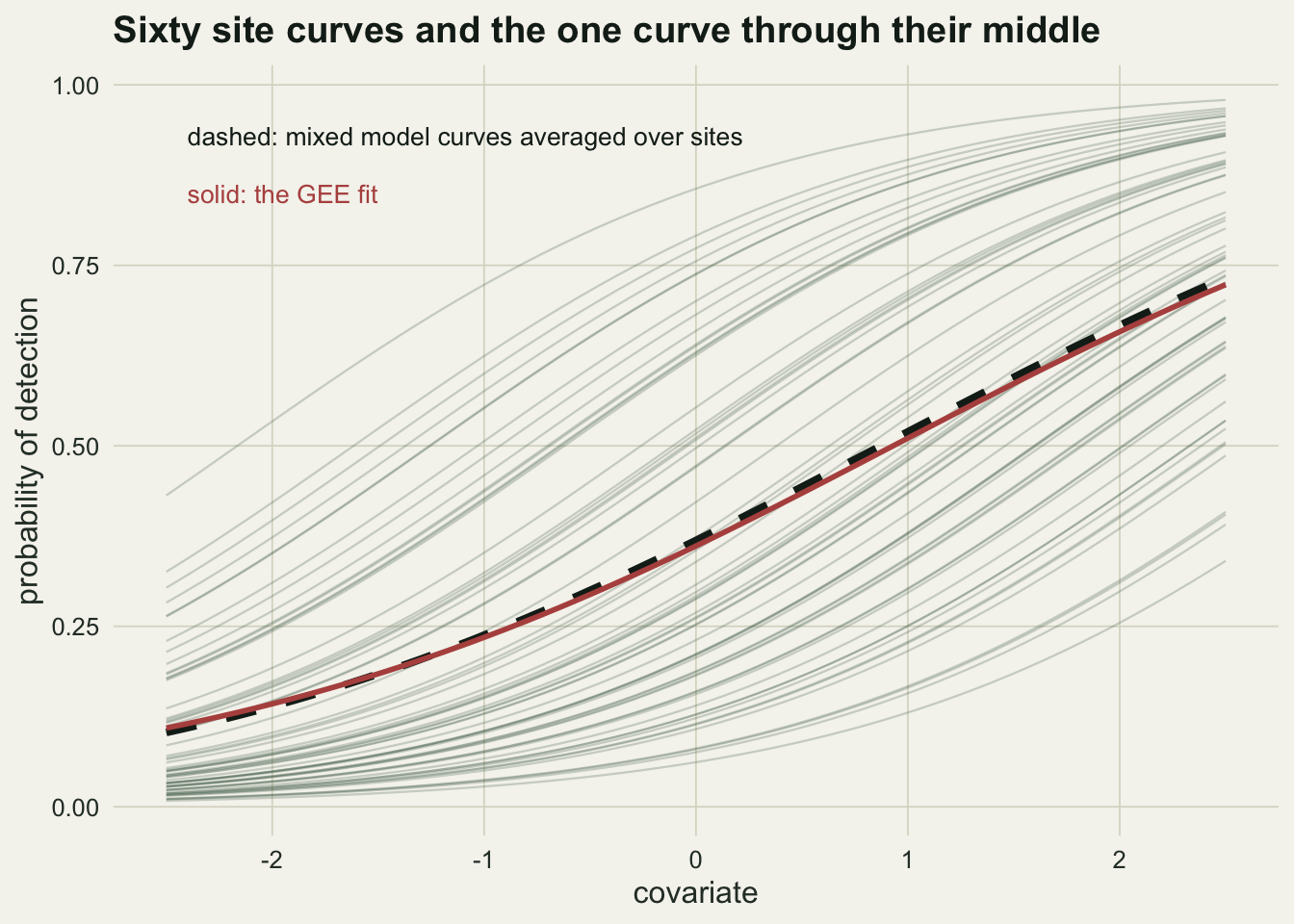
The logistic curve is not a straight line, so averaging over sites is not the same as averaging inside them. Each site has its own curve, shifted left or right by its random intercept. Average those curves at each value of the predictor and the result is flatter than any of them, because the steep parts of different sites land at different places on the x axis and the flat tails fill in the rest.
There is a standard approximation for how much flatter. Multiply the conditional slope by one over the square root of one plus 0.346 times the between-site variance.
```{r attenuation}
s <- sqrt(unlist(VarCorr(m_glmm))[[1]])
round(c(observed_ratio = coef(m_gee)[["x"]] / fixef(m_glmm)[["x"]],
        approximation  = (1 + 0.346 * s^2)^(-0.5)), 3)
```
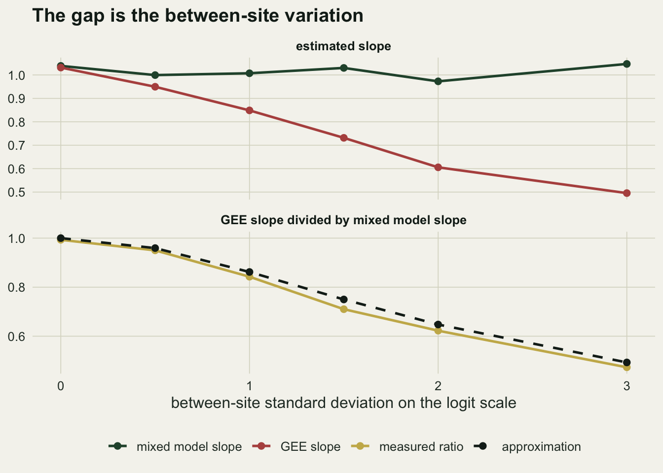
The relationship is not a rule of thumb about one data set. Sweep the between-site standard deviation and it holds across the range.
```{r sweep}
#| warning: false
one_rep <- function(sigma) {
  dd <- sim_binary(sigma = sigma)
  g  <- glmer(y ~ x + (1 | site), family = binomial, data = dd)
  e  <- geeglm(y ~ x, id = site, family = binomial, corstr = "exchangeable",
               data = dd[order(dd$site), ])
  c(glmm = fixef(g)[["x"]], gee = coef(e)[["x"]])
}
sigmas <- c(0, 0.5, 1, 1.5, 2, 3)
set.seed(9)
sw <- t(vapply(sigmas, function(s0) rowMeans(replicate(30, one_rep(s0))),
               numeric(2)))
sweep_tab <- data.frame(sigma = sigmas, glmm = sw[, 1], gee = sw[, 2],
                        ratio = sw[, 2] / sw[, 1],
                        approx = (1 + 0.346 * sigmas^2)^(-0.5))
round(sweep_tab, 3)
```
The conditional slope stays near the generating value of 1 at every level of between-site variation, which is what it should do. The marginal slope falls away from it, and the approximation tracks the fall. It is an approximation, and it sits above the measured ratio at every level here, by at most `r sprintf("%.3f", max(sweep_tab$approx - sweep_tab$ratio))`.
```{r fig-attenuation}
#| fig-cap: "Mean estimated slope against the between-site standard deviation, for the mixed model and the GEE, with the standard approximation to the ratio."
#| fig-alt: "Two panels sharing an x axis of between-site standard deviation. In the upper panel the mixed model slope stays level near one across the whole range, while the GEE slope starts at the same height and drops away steadily. In the lower panel one line gives the GEE slope divided by the mixed model slope, running from one down to about one half, and a dashed line for the approximation sits just above it in a different colour."
top <- rbind(
  data.frame(sigma = sigmas, value = sweep_tab$glmm, what = "mixed model slope"),
  data.frame(sigma = sigmas, value = sweep_tab$gee,  what = "GEE slope"))
bot <- rbind(
  data.frame(sigma = sigmas, value = sweep_tab$ratio,  what = "measured ratio"),
  data.frame(sigma = sigmas, value = sweep_tab$approx, what = "approximation"))
top$panel <- "estimated slope"
bot$panel <- "GEE slope divided by mixed model slope"
both <- rbind(top, bot)
both$panel <- factor(both$panel, levels = unique(both$panel))
both$what  <- factor(both$what, levels = c("mixed model slope", "GEE slope",
                                           "measured ratio", "approximation"))

ggplot(both, aes(x = sigma, y = value, colour = what, linetype = what)) +
  geom_line(linewidth = 0.9) +
  geom_point(size = 2) +
  facet_wrap(~ panel, ncol = 1, scales = "free_y") +
  scale_colour_manual(values = c(te_forest, te_rust, te_gold, te_ink)) +
  scale_linetype_manual(values = c("solid", "solid", "solid", "dashed")) +
  labs(x = "between-site standard deviation on the logit scale",
       y = NULL, colour = NULL, linetype = NULL,
       title = "The gap is the between-site variation") +
  theme_datasheet() +
  theme(legend.position = "bottom",
        strip.text = element_text(colour = te_ink, face = "bold"))
```
## The GEE curve is the average of the mixed model curves
That is a claim about shapes, so it can be checked directly. Take the fitted mixed model, integrate its curve over the estimated distribution of site intercepts, and compare the result with the GEE's fitted curve. They were estimated by different machinery from the same data, so agreement is not built in.
```{r marginalise}
b  <- fixef(m_glmm)
xs <- seq(-2.5, 2.5, length.out = 60)
marginal_of_glmm <- vapply(xs, function(xx)
  integrate(function(u) plogis(b[[1]] + b[[2]] * xx + u) * dnorm(u, 0, s),
            -6 * s, 6 * s)$value, numeric(1))
gee_fit <- plogis(coef(m_gee)[[1]] + coef(m_gee)[[2]] * xs)

round(c(largest_gap = max(abs(gee_fit - marginal_of_glmm)),
        at_x_zero_gee = gee_fit[which.min(abs(xs))],
        at_x_zero_integrated = marginal_of_glmm[which.min(abs(xs))]), 4)
```
```{r fig-curves}
#| fig-cap: "Fitted probability of detection against the covariate: one curve per site from the mixed model, their average, and the GEE fit."
#| fig-alt: "Many pale rising curves fanned out across the plot, one per site, together covering almost the whole range from zero to one. A thick dashed curve runs through the middle of them with a visibly gentler slope, and a solid curve of a different colour lies almost exactly on top of the dashed one."
site_u <- ranef(m_glmm)$site[, 1]
per_site <- do.call(rbind, lapply(seq_along(site_u), function(i)
  data.frame(x = xs, p = plogis(b[[1]] + b[[2]] * xs + site_u[i]), site = i)))
avg <- data.frame(x = xs, p = marginal_of_glmm)
gee <- data.frame(x = xs, p = gee_fit)

ggplot() +
  geom_line(data = per_site, aes(x = x, y = p, group = site),
            colour = te_forest, alpha = 0.22, linewidth = 0.4) +
  geom_line(data = avg, aes(x = x, y = p), colour = te_ink,
            linewidth = 1.4, linetype = "dashed") +
  geom_line(data = gee, aes(x = x, y = p), colour = te_rust, linewidth = 1) +
  annotate("text", x = -2.4, y = 0.93, hjust = 0, size = 3.5, colour = te_ink,
           label = "dashed: mixed model curves averaged over sites") +
  annotate("text", x = -2.4, y = 0.85, hjust = 0, size = 3.5, colour = te_rust,
           label = "solid: the GEE fit") +
  labs(x = "covariate", y = "probability of detection",
       title = "Sixty site curves and the one curve through their middle") +
  theme_datasheet()
```
## On a log link the slopes agree and the intercept does not
The attenuation is a property of the logit link, not of clustering. Repeat the exercise with counts and a log link.
```{r poisson}
#| warning: false
sim_pois <- function(n_site = 60, n_visit = 12, sigma = 0.8, beta = 0.5) {
  site <- rep(seq_len(n_site), each = n_visit)
  u <- rnorm(n_site, 0, sigma)[site]
  x <- rnorm(n_site * n_visit)
  data.frame(site = factor(site), x = x,
             y = rpois(length(x), exp(0.8 + beta * x + u)))
}
set.seed(20260812)
dp <- sim_pois()
p_glmm <- glmer(y ~ x + (1 | site), family = poisson, data = dp)
p_gee  <- geeglm(y ~ x, id = site, family = poisson, corstr = "exchangeable",
                 data = dp[order(dp$site), ])

round(c(glmm_slope     = fixef(p_glmm)[["x"]],
        gee_slope      = coef(p_gee)[["x"]],
        glmm_intercept = fixef(p_glmm)[[1]],
        gee_intercept  = coef(p_gee)[[1]],
        half_variance  = unlist(VarCorr(p_glmm))[[1]] / 2), 3)
```
The two slopes agree, because exponentials multiply: a shift in the intercept scales every site's expected count by the same factor and leaves the slope alone. The intercepts do not agree, and the size of the gap is not arbitrary. Averaging `exp(u)` over a normal `u` gives `exp(sigma^2 / 2)`, so the marginal intercept should sit above the conditional one by half the between-site variance. Here the measured gap is `r sprintf("%.3f", coef(p_gee)[[1]] - fixef(p_glmm)[[1]])` against a half-variance of `r sprintf("%.3f", unlist(VarCorr(p_glmm))[[1]] / 2)`.
This is the sentence to keep: on a log link, a conditional rate ratio is also a marginal rate ratio, and a conditional mean is not a marginal mean.
## What the GEE is really buying
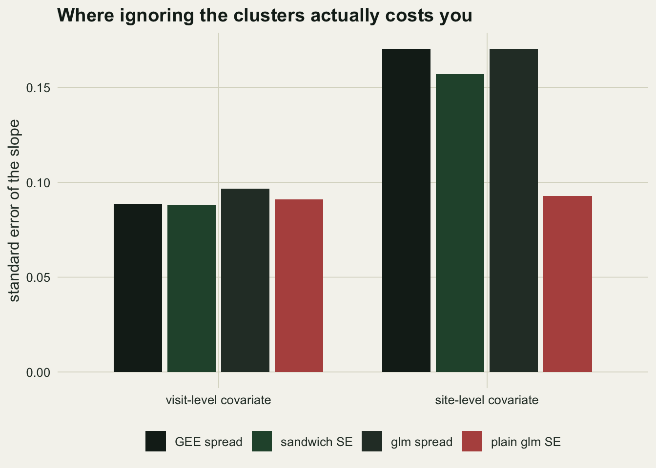
The sandwich estimator is the part of a GEE that earns its keep, and it earns it in a specific place. Compare three quantities across 300 simulated data sets: the actual spread of the estimate, the sandwich standard error, and the standard error a plain `glm` reports when the clustering is ignored. Do it once for a covariate that varies visit to visit and once for a covariate measured at the site.
```{r sandwich}
sim_level <- function(level, n_site = 60, n_visit = 12, sigma = 1.2, beta = 1) {
  site <- rep(seq_len(n_site), each = n_visit)
  u <- rnorm(n_site, 0, sigma)[site]
  x <- if (level == "site") rnorm(n_site)[site] else rnorm(n_site * n_visit)
  data.frame(site = factor(site), x = x,
             y = rbinom(length(x), 1, plogis(-0.3 + beta * x + u)))
}
one_se <- function(level) {
  dd <- sim_level(level)
  dd <- dd[order(dd$site), ]
  g  <- geeglm(y ~ x, id = site, family = binomial, corstr = "exchangeable",
               data = dd)
  gi <- glm(y ~ x, family = binomial, data = dd)
  c(gee_est = coef(g)[["x"]],   sandwich = coef(summary(g))[2, 2],
    glm_est = coef(gi)[["x"]],  naive    = coef(summary(gi))[2, 2])
}
se_tab <- do.call(rbind, lapply(c("visit", "site"), function(lv) {
  set.seed(55)
  R <- t(replicate(300, one_se(lv)))
  # each standard error is compared with the spread of ITS OWN estimator
  data.frame(covariate    = lv,
             gee_spread   = sd(R[, "gee_est"]),   # equal to glm_spread for a site-level
                                                  # covariate with balanced clusters
             sandwich     = mean(R[, "sandwich"]),
             glm_spread   = sd(R[, "glm_est"]),
             naive_glm    = mean(R[, "naive"]))
}))
se_tab$naive_over_true <- se_tab$naive_glm / se_tab$glm_spread
data.frame(covariate = se_tab$covariate,
           round(se_tab[, -1], 4))
```
For the visit-level covariate the plain `glm` standard error is `r sprintf("%.2f", se_tab$naive_over_true[1])` times the actual spread of the `glm` estimate, which is to say it is nearly right. Clustering did not cost much there, because each site contributes its own within-site contrast. For the site-level covariate the plain standard error is `r sprintf("%.2f", se_tab$naive_over_true[2])` times the truth: confidence intervals a little over half as wide as they should be, on the covariate whose effect is usually the point of the study. The sandwich gets close to the spread of its own estimator in both cases, a shade low for the site-level one.
That is the practical rule. Ignoring clustering damages the standard error of the covariate measured at the cluster level far more than the one measured within it, and the folklore that treats all clustered data as equally dangerous makes the wrong repairs.
```{r fig-se}
#| fig-cap: "Spread of each estimated slope over 300 data sets, against the standard error that claims to describe it. Each standard error is paired with its own estimator."
#| fig-alt: "A grouped bar chart with two groups on the x axis, visit-level and site-level covariate. Within each group, four bars in two pairs: the spread of the GEE estimate beside its sandwich standard error, and the spread of the glm estimate beside the plain glm standard error. In the visit-level group all four bars are close to the same height. In the site-level group both spreads are tall, the sandwich almost matches them, and the plain glm standard error is little more than half their height."
bars <- data.frame(
  covariate = rep(c("visit-level covariate", "site-level covariate"), each = 4),
  what = rep(c("GEE spread", "sandwich SE", "glm spread", "plain glm SE"), 2),
  value = c(se_tab$gee_spread[1], se_tab$sandwich[1],
            se_tab$glm_spread[1], se_tab$naive_glm[1],
            se_tab$gee_spread[2], se_tab$sandwich[2],
            se_tab$glm_spread[2], se_tab$naive_glm[2]))
bars$covariate <- factor(bars$covariate,
                         levels = c("visit-level covariate", "site-level covariate"))
bars$what <- factor(bars$what,
                    levels = c("GEE spread", "sandwich SE",
                               "glm spread", "plain glm SE"))

ggplot(bars, aes(x = covariate, y = value, fill = what)) +
  geom_col(position = position_dodge(width = 0.8), width = 0.72) +
  scale_fill_manual(values = c(te_forest, "#8fae94", te_gold, te_rust)) +
  labs(x = NULL, y = "standard error of the slope", fill = NULL,
       title = "Where ignoring the clusters actually costs you") +
  theme_datasheet() +
  theme(legend.position = "bottom")
```
## What a GEE cannot do
It has no site-level estimates, so there is nothing to map or predict for a named site, and no variance component, so it cannot say how much of the variation is between sites. Random slopes, nested levels and partial pooling of small sites towards the mean are all outside it. There is no likelihood either, so model comparison runs on QIC rather than AIC and there is no likelihood ratio test.
It also needs enough clusters. The sandwich is an asymptotic result in the number of clusters, not the number of observations, and with fewer than about forty it becomes optimistic; small-sample corrections exist and should be used rather than skipped. Sixty sites here is comfortable, and the sandwich still sits a little below the true spread for the site-level covariate.
Against that, a GEE fits when a GLMM will not. It has no likelihood to maximise over a random-effect distribution, so there is no boundary to hit and no singular fit, and it does not assume the site effects are normal.
## Honest limits
Everything above uses a random intercept only. With random slopes the conditional and marginal effects still differ, the difference is no longer a single scalar factor, and the approximation used here does not apply.
The 0.346 constant comes from approximating the logistic function by a probit, and it is good rather than exact. The table shows it slightly overstating the ratio at the larger variances, and it says nothing at all about links other than the logit.
The two estimators also differ in what they assume about missing data, and the difference favours the mixed model. A GEE is a moment-based estimator and needs the missingness to be completely at random, or to be corrected by inverse-probability weights. A likelihood-based GLMM is valid under the weaker condition that whether a visit happened depends only on things that were observed and are in the model, such as whether the species was detected at earlier visits to the same site. Repeat-visit data is full of exactly that, and a GEE fitted to it without weights is using an assumption the design does not support. Neither estimator survives missingness that depends on what the missed visit would have found.
The simulation generates data from exactly the model the GLMM fits, which is the friendliest possible case for it. Under a misspecified random-effect distribution the conditional estimate can be biased while the marginal one is not, and that asymmetry is a real argument for GEEs that this post has not measured.
Finally, the choice framed here as marginal against conditional is only sharp for a nonlinear link. For an ordinary linear model with an identity link the two coincide, which is why the distinction never comes up until the first logistic regression.
## References
Zeger SL, Liang KY, Albert PS 1988 Biometrics 44(4):1049-1060 (10.2307/2531734)
Halekoh U, Hojsgaard S, Yan J 2006 Journal of Statistical Software 15(2):1-11 (10.18637/jss.v015.i02)
Bates D, Machler M, Bolker B, Walker S 2015 Journal of Statistical Software 67(1):1-48 (10.18637/jss.v067.i01)
## Related tutorials
- [GLMMs for nested counts](../glmm-nested-counts-pseudoreplication/)
- [Marginal vs conditional R-squared](../marginal-vs-conditional-r2/)
- [Per chick or per nest: informative cluster size](../informative-cluster-size/)
- [Pseudoreplication in ecology](../pseudoreplication-in-ecology/)