---
title: "The Moran process and fixation probability"
description: "Model selection in a finite population in base R: the Moran birth-death process, the exact fixation probability of a single mutant, and how long fixation takes."
date: "2026-07-09 12:00"
date-modified: "2026-10-08"
categories: [evolutionary ecology, population dynamics, natural selection, R, ecology tutorial]
image: thumbnail.png
image-alt: "Fixation probability rising with mutant fitness for three population sizes, with the large-population limit drawn as a dashed curve"
---
*Corrected 8 October 2026: the post explained why a single selected mutant takes longer to absorb than a neutral one by its surviving runs having further to travel, and now gives the real reason, that a much larger share of selected runs go on to fix and a run that fixes is slow; it also said a mutant at ten copies is already past the dangerous phase, and now says how often such a mutant is still lost.*
*Corrected 30 September 2026: the post said population size stops mattering almost immediately above a relative fitness of one; it now says the two larger populations coincide while the smallest stays above them by a shrinking margin.*
Every model in the last few posts assumed an infinite population. The replicator equation tracks frequencies, frequencies change smoothly, and a strategy with higher payoff always increases. Real populations are finite, and in a finite population the fitter type sometimes disappears anyway, because the individual carrying it happened to die before reproducing.
That is not a small correction. In a population of 100, a mutant with a ten per cent fitness advantage fixes about nine times in a hundred and vanishes the other ninety-one. Selection is still doing its work: nine per cent is nine times the neutral rate. But the modal outcome for a beneficial mutation is loss, and no deterministic model can say that.
The Moran process is the smallest model that gets this right. It has one parameter beyond the population size, it can be written in ten lines, and its fixation probability has a closed form that you can check against simulation.
## The model
Fix the population size at `N` individuals, each of one of two types: `A` with fitness `r`, and `B` with fitness 1. One elementary step does two things at once. An individual is chosen to reproduce, with probability proportional to fitness, and its offspring replaces an individual chosen uniformly at random to die. The population size never changes, and generations overlap completely.
If there are `i` copies of `A`, the total fitness is `ri + (N - i)`. The count goes up when an `A` reproduces and a `B` dies, and down when a `B` reproduces and an `A` dies:
$$p_{i,i+1} = \frac{ri}{ri + N - i} \cdot \frac{N-i}{N}, \qquad p_{i,i-1} = \frac{N-i}{ri + N - i} \cdot \frac{i}{N}$$
Everything else is the probability of staying put. States 0 and `N` are absorbing: once a type is gone it cannot come back, because there is no mutation.
That structure makes the fixation probability a standard birth-death calculation. Writing $\gamma_i = p_{i,i-1}/p_{i,i+1} = 1/r$, which does not depend on `i` here, the probability that a single `A` takes over is
$$\rho_1 = \frac{1 - r^{-1}}{1 - r^{-N}}$$
and the general starting point `i` gives $(1 - r^{-i})/(1 - r^{-N})$. At `r` exactly 1 the expression is 0/0 and the limit is `i/N`, which is the neutral result: a mutant fixes with the frequency it starts at.
```{r}
#| label: exact
rho <- function(r, N, i = 1) if (r == 1) i / N else (1 - r^-i) / (1 - r^-N)

for (r in c(0.90, 0.99, 1.00, 1.01, 1.10, 1.50, 2.00)) {
  cat(sprintf("r = %.2f   rho_1 = %-11.6g   1 - 1/r = %s\n",
              r, rho(r, 100),
              if (r > 1) sprintf("%.6g", 1 - 1 / r) else "not defined"))
}
```
Three things in that table are worth stopping on.
A ten per cent advantage buys a fixation probability of `r sprintf("%.6g", rho(1.1, 100))` in a population of 100, against a neutral `r sprintf("%.6g", rho(1, 100))`. Selection multiplied the mutant's chances by nine, and still lost nine times out of ten.
A ten per cent disadvantage does not give zero. It gives $2.95134 \times 10^{-6}$, which is small but not impossible, and in a large population of such mutants it happens. Deleterious variants do fix.
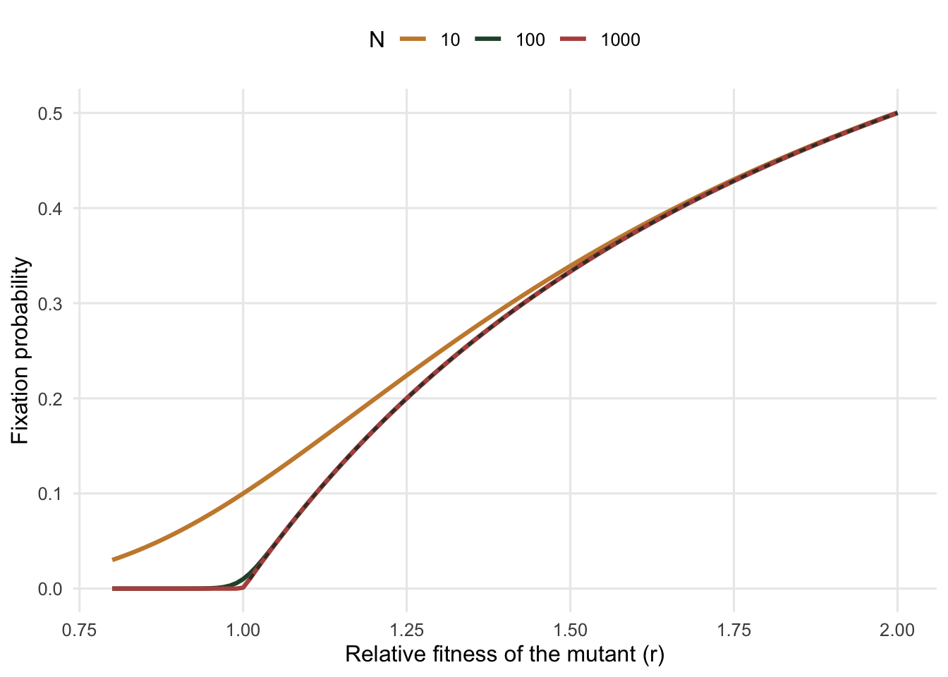
For `r` above about 1.1 the exact answer and the large-population limit `1 - 1/r` agree to four decimal places at `N` = 100. That limit is the number worth memorising: a mutant with a ten per cent advantage fixes about a tenth of the time, whatever the population size, once the population is not tiny. The agreement breaks down for weak selection, where `r` = 1.01 gives `r sprintf("%.6g", rho(1.01, 100))` against a limit of `r sprintf("%.6g", 1 - 1 / 1.01)`, because the relevant quantity is `N(r - 1)` rather than the selection coefficient on its own, and here that product is only 1.
## A simulation check
The formula is short enough to be wrong in a way that looks right, so run the process itself. Each replicate walks until it hits 0 or `N`, and the fraction ending at `N` estimates $\rho_1$. The binomial standard error over 2000 replicates is about `r sprintf("%.4f", sqrt(rho(1.1, 100) * (1 - rho(1.1, 100)) / 2000))` near a probability of `r sprintf("%.2f", rho(1.1, 100))`, so agreement to within a couple of standard errors is all that can be asked.
```{r}
#| label: simulate
sim_moran <- function(r, N, i0 = 1, reps = 2000, seed = 1) {
  set.seed(seed)
  hits <- 0L
  for (m in seq_len(reps)) {
    i <- i0
    while (i > 0 && i < N) {
      fa <- r * i; fb <- N - i; tot <- fa + fb
      pup <- (fa / tot) * ((N - i) / N)
      pdn <- (fb / tot) * (i / N)
      u <- runif(1)
      if (u < pup) i <- i + 1L else if (u < pup + pdn) i <- i - 1L
    }
    if (i == N) hits <- hits + 1L
  }
  hits / reps
}

cfg <- data.frame(r = c(1.1, 1.0), seed = c(1, 2))
for (k in seq_len(nrow(cfg))) {
  rr <- cfg$r[k]
  p  <- sim_moran(rr, 100, reps = 2000, seed = cfg$seed[k])
  ex <- rho(rr, 100)
  err <- sqrt(ex * (1 - ex) / 2000)
  cat(sprintf("r = %.2f   simulated %.4f   exact %.7f   se %.5f   gap %.2f se\n",
              rr, p, ex, err, abs(p - ex) / err))
}
```
Both land inside one standard error. That is the check that matters, and it also shows why simulating this model to answer a fine question is a poor use of a processor: distinguishing `r` = 1.01 from neutrality means separating `r sprintf("%.4f", rho(1.01, 100))` from `r sprintf("%.4f", rho(1, 100))`, a gap of `r sprintf("%.4f", rho(1.01, 100) - rho(1, 100))` that is only about two standard errors of a 2000 replicate estimate of the larger value, so a run of that size cannot call it reliably.
## The shape of the curve
```{r}
#| label: fig-rho
#| fig-cap: "Fixation probability of a single mutant against its relative fitness, for three population sizes. The dashed curve is the large-population limit 1 - 1/r, which the N = 100 and N = 1000 curves sit on top of above about r = 1.1."
#| fig-alt: "Three rising curves of fixation probability against relative fitness; the two larger population sizes coincide with a dashed reference curve while the smallest starts well above it and closes on it as fitness grows"
library(ggplot2)
te_canvas <- theme(plot.background  = element_rect(fill = "#f5f4ee", colour = NA),
                   panel.background = element_rect(fill = "#f5f4ee", colour = NA))
rs <- seq(0.8, 2, by = 0.01)
curves <- do.call(rbind, lapply(c(10, 100, 1000), function(N)
  data.frame(r = rs, N = factor(N), p = sapply(rs, rho, N = N))))
lim <- data.frame(r = rs[rs > 1], p = 1 - 1 / rs[rs > 1])

ggplot(curves, aes(r, p, colour = N)) +
  geom_line(linewidth = 1.1) +
  geom_line(data = lim, aes(r, p), inherit.aes = FALSE,
            colour = "#3a3a33", linetype = "22", linewidth = 0.8) +
  scale_colour_manual(values = c(`10` = "#c98a3a", `100` = "#275139",
                                 `1000` = "#b5534e")) +
  labs(x = "Relative fitness of the mutant (r)", y = "Fixation probability",
       colour = "N") +
  theme_minimal(base_size = 12) + te_canvas +
  theme(legend.position = "top", panel.grid.minor = element_blank())
```
Below `r` = 1 the curves separate sharply and the large population is the harshest: a deleterious mutant in a population of 1000 is essentially certain to be lost, while in a population of 10 it has a real chance. Above `r` = 1 the curves for 100 and 1000 coincide almost immediately; the `N` = 10 curve stays above them, partly because its neutral starting value `1/N` is higher, but by a margin that shrinks as `r` grows and is small, in relative terms, beside the differences between the curves below one, which run to orders of magnitude. This asymmetry is the whole reason effective population size appears in every discussion of molecular evolution. Big populations are efficient at removing bad variants and no better than small ones at spreading good variants.
The `N` = 10 curve staying above the others on the left is drift protecting deleterious mutations, and it is the same effect that lets nearly neutral theory work: whether a mutation behaves as neutral depends on `Ns`, not on `s`.
## Trajectories
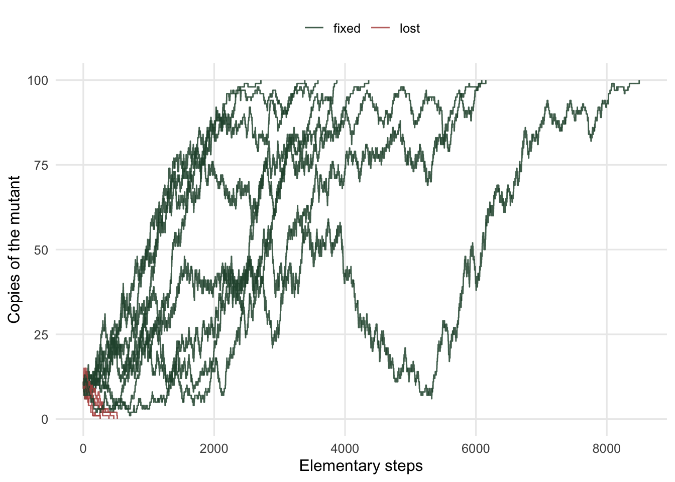
The averages hide what individual runs look like. Twelve replicates starting from ten copies, with a ten per cent advantage:
```{r}
#| label: fig-paths
#| fig-cap: "Twelve independent runs of the Moran process at r = 1.1 in a population of 100, each starting from ten copies of the mutant. Runs are coloured by their outcome."
#| fig-alt: "Twelve jagged random walk paths of mutant count against time; four fall to zero early while eight climb and reach the population size"
traj <- function(r, N, i0, seed, maxstep = 60000) {
  set.seed(seed)
  out <- integer(maxstep); i <- i0; k <- 0L
  while (k < maxstep) {
    k <- k + 1L; out[k] <- i
    if (i == 0 || i == N) break
    fa <- r * i; fb <- N - i; tot <- fa + fb
    pup <- (fa / tot) * ((N - i) / N)
    pdn <- (fb / tot) * (i / N)
    u <- runif(1)
    if (u < pup) i <- i + 1L else if (u < pup + pdn) i <- i - 1L
  }
  out[seq_len(k)]
}

runs <- do.call(rbind, lapply(1:12, function(s) {
  v <- traj(1.1, 100, 10, seed = s)
  data.frame(run = factor(s), step = seq_along(v), i = v,
             fate = if (v[length(v)] == 100) "fixed" else "lost")
}))
cat("fixed:", length(unique(runs$run[runs$fate == "fixed"])), "of 12",
    " exact probability from i = 10:", sprintf("%.4f", rho(1.1, 100, 10)), "\n")
ggplot(runs, aes(step, i, group = run, colour = fate)) +
  geom_step(linewidth = 0.5, alpha = 0.85) +
  scale_colour_manual(values = c(fixed = "#275139", lost = "#b5534e")) +
  labs(x = "Elementary steps", y = "Copies of the mutant", colour = NULL) +
  theme_minimal(base_size = 12) + te_canvas +
  theme(legend.position = "top", panel.grid.minor = element_blank())
```
Eight of the twelve fixed, against an exact probability of `r sprintf("%.4f", rho(1.1, 100, 10))` from ten copies. Starting from ten rather than one has changed the problem: a mutant that reaches ten copies has come through the most dangerous phase, though it is still lost about `r sprintf("%.0f", 100 * (1 - rho(1.1, 100, 10)))` times in a hundred, and the fixation probability jumped from `r sprintf("%.2f", rho(1.1, 100))` to `r sprintf("%.2f", rho(1.1, 100, 10))`.
The lost runs are short and the surviving ones are long, which is the usual pattern and the reason a plot of "typical" trajectories from a fixed time budget is misleading. Failure is quick.
## How long does it take?
Fixation probability answers whether, not when. The expected number of steps to absorption from state `i` satisfies
$$t_i = 1 + p_{i,i-1}\,t_{i-1} + p_{i,i+1}\,t_{i+1} + (1 - p_{i,i-1} - p_{i,i+1})\,t_i$$
with $t_0 = t_N = 0$. Rearranged, that is a tridiagonal linear system in the `N - 1` interior states, which `solve` handles directly. No simulation, no approximation.
```{r}
#| label: fig-time
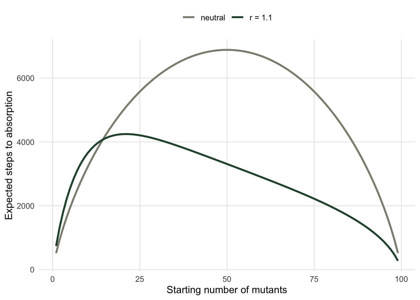
#| fig-cap: "Expected number of elementary steps to absorption against the starting number of mutants, in a population of 100, for a neutral mutant and one with a ten per cent advantage."
#| fig-alt: "Two humped curves of expected absorption time against starting mutant count; the neutral curve peaks near the middle at about 6900 steps; the selected curve peaks earlier, near 20 starting mutants, at about 4200 steps, and lies slightly above the neutral curve for the smallest starting counts"
abs_time <- function(r, N) {
  pup <- function(i) (r * i) / (r * i + N - i) * (N - i) / N
  pdn <- function(i) (N - i) / (r * i + N - i) * i / N
  A <- matrix(0, N - 1, N - 1); b <- rep(-1, N - 1)
  for (i in 1:(N - 1)) {
    A[i, i] <- -(pup(i) + pdn(i))
    if (i > 1)     A[i, i - 1] <- pdn(i)
    if (i < N - 1) A[i, i + 1] <- pup(i)
  }
  solve(A, b)
}

t_neu <- abs_time(1.0, 100)
t_sel <- abs_time(1.1, 100)
cat(sprintf("neutral   from i = 1: %9.4f steps    from i = 50: %9.4f\n",
            t_neu[1], t_neu[50]))
cat(sprintf("r = 1.1   from i = 1: %9.4f steps    from i = 50: %9.4f\n",
            t_sel[1], t_sel[50]))
cat(sprintf("diffusion approximation for the neutral midpoint, N^2 log 2 = %.4f\n",
            100^2 * log(2)))
times <- rbind(
  data.frame(i = 1:99, steps = t_neu, model = "neutral"),
  data.frame(i = 1:99, steps = t_sel, model = "r = 1.1"))
ggplot(times, aes(i, steps, colour = model)) +
  geom_line(linewidth = 1.1) +
  scale_colour_manual(values = c(neutral = "#8d8d80", "r = 1.1" = "#275139")) +
  labs(x = "Starting number of mutants", y = "Expected steps to absorption",
       colour = NULL) +
  theme_minimal(base_size = 12) + te_canvas +
  theme(legend.position = "top", panel.grid.minor = element_blank())
```
The neutral midpoint takes `r sprintf("%.4f", t_neu[50])` steps against a diffusion prediction of `r sprintf("%.4f", 100^2 * log(2))`, an agreement of better than one per cent from a formula that assumes `N` is large and 100 is not especially large. Divide by `N` to get generations in the usual sense and the neutral midpoint is about `r round(t_neu[50] / 100)` generations, which for most organisms is nothing.
Selection cuts the midpoint time roughly in half, to `r sprintf("%.4f", t_sel[50])`. Starting from a single copy the ordering reverses: the selected mutant takes `r sprintf("%.4f", t_sel[1])` steps against the neutral `r sprintf("%.4f", t_neu[1])`, because a much larger share of selected runs go on to fix, and a run that fixes takes far longer than one that is lost. Conditioning changes the answer, and unconditional expected times mix two very different populations of runs.
## An honest limit
The Moran process buys its closed form with assumptions that are all worth naming.
Population size is fixed. Nothing about a real population holds `N` constant to the individual, and the fixation probability depends on `N` only through `r^-N`, so for a mutant with `r` comfortably above 1 the result is not sensitive to the exact value; but a population that crashes and recovers behaves like the smaller size for drift purposes, which is what effective population size is trying to capture. Feeding a census count into these formulas will overstate the efficiency of selection, often by an order of magnitude.
Generations overlap completely, one birth and one death at a time. The Wright-Fisher model makes the opposite choice, replacing the whole population at once, and gives $\rho_1 \approx (1 - e^{-2s})/(1 - e^{-2Ns})$ with `s` = `r` - 1, differing from the Moran answer by a factor of two in the exponent. Neither is more correct in general. The factor of two is a modelling choice about life history that is easy to lose track of when comparing published numbers.
Fitness is constant. The whole apparatus assumes `r` does not depend on how common the type is, which rules out every frequency-dependent case, and those are the interesting ones in behaviour and in competition. That extension is the subject of the next post.
There is no mutation. Absorbing states are absorbing only because nothing regenerates the lost type. With recurrent mutation the process has a stationary distribution instead, and "fixation probability" becomes a statement about the rate of transitions between mostly-`A` and mostly-`B` states rather than a final outcome.
The population is well mixed, every individual competing with every other. [Network reciprocity on a lattice](../network-reciprocity-on-a-lattice/) showed how much structure can change a conclusion, and structure changes fixation probabilities too.
## References
Moran 1958 Mathematical Proceedings of the Cambridge Philosophical Society 54(1):60-71 (10.1017/S0305004100033193)
Kimura 1962 Genetics 47(6):713-719 (10.1093/genetics/47.6.713)
Nowak 2006 "Evolutionary Dynamics: Exploring the Equations of Life" ISBN 978-0674023383
Ewens 2004 "Mathematical Population Genetics 1: Theoretical Introduction" ISBN 978-0387201917
## Related tutorials
- [Evolutionary games in finite populations](../games-in-finite-populations/)
- [The replicator equation](../the-replicator-equation/)
- [Checking a finite population model](../checking-a-finite-population-model/)
- [Adaptive dynamics and evolutionary branching](../adaptive-dynamics-and-branching/)