---
title: "Life-history trade-offs in R"
description: "Life-history trade-offs in R: the cost of reproduction, the optimal reproductive effort, and Cole's paradox on why iteroparity pays when juveniles die young."
date: "2026-07-01 13:00"
categories: [ecology tutorial, R, life history, evolutionary ecology, population ecology]
image: thumbnail.png
image-alt: "Fecundity rising and adult survival falling with reproductive effort, and a lifetime-output curve peaking at an intermediate effort."
---
```{r setup}
#| code-fold: true
#| code-summary: "Setup: packages, colours and plot theme"
#| results: hide
#| message: false
#| warning: false
knitr::opts_chunk$set(echo = TRUE, message = FALSE, warning = FALSE,
                      dev = "png", dpi = 120, fig.path = "figures/",
                      fig.width = 7, fig.height = 4.4)
library(ggplot2)
theme_te <- theme_minimal(base_size = 12) +
  theme(panel.background = element_rect(fill = "#f5f4ee", colour = NA),
        plot.background  = element_rect(fill = "#f5f4ee", colour = NA),
        panel.grid.minor = element_blank(),
        plot.title = element_text(face = "bold", size = 12))
theme_set(theme_te)
col_fec <- "#b5651d"; col_sur <- "#3a6b52"; col_fit <- "#333333"; col_ref <- "#555555"

fmax <- 6; smax <- 0.85
fec <- function(E) fmax * E^0.7
sur <- function(E) smax * (1 - E)^0.6
R0  <- function(E) fec(E) / (1 - sur(E))
Es <- seq(0.01, 0.99, 0.001); Estar <- Es[which.max(R0(Es))]; R0star <- max(R0(Es))
R0_semel <- fec(1)
juv <- 0.1; adult <- 0.8; cole_extra <- adult/juv
```
Every organism runs on a finite budget, and life-history theory is the economics of spending it. Energy and time put into reproduction now cannot go into growth, maintenance, or reproduction later. That constraint, the principle of allocation, forces trade-offs, and the shape of those trade-offs decides how many offspring to have, when to have them, and whether to breed once or many times (Stearns 1989 Functional Ecology 3(3):259-268).
## The cost of reproduction
Fix the central trade-off: reproductive effort against survival. Put more into this year's brood and you raise fecundity but lower your own chance of living to breed again. Write fecundity as rising with effort `E` and adult survival as falling with it.
```{r tradeoff}
fmax <- 6; smax <- 0.85
fec <- function(E) fmax * E^0.7          # fecundity rises with effort
sur <- function(E) smax * (1 - E)^0.6    # adult survival falls with effort
R0  <- function(E) fec(E) / (1 - sur(E)) # lifetime output for a simple iteroparous life
c(effort_low = R0(0.2), effort_mid = R0(0.45), effort_high = R0(0.9))
```
Lifetime reproductive output, `R0`, sums this year's brood over all the years the adult survives, which for constant annual survival is `fecundity / (1 - survival)`. Maximise it over effort.
```{r optimum}
Es <- seq(0.01, 0.99, 0.001)
Estar <- Es[which.max(R0(Es))]
c(optimal_effort = Estar, R0_at_optimum = R0(Estar), R0_if_semelparous = fec(1))
```
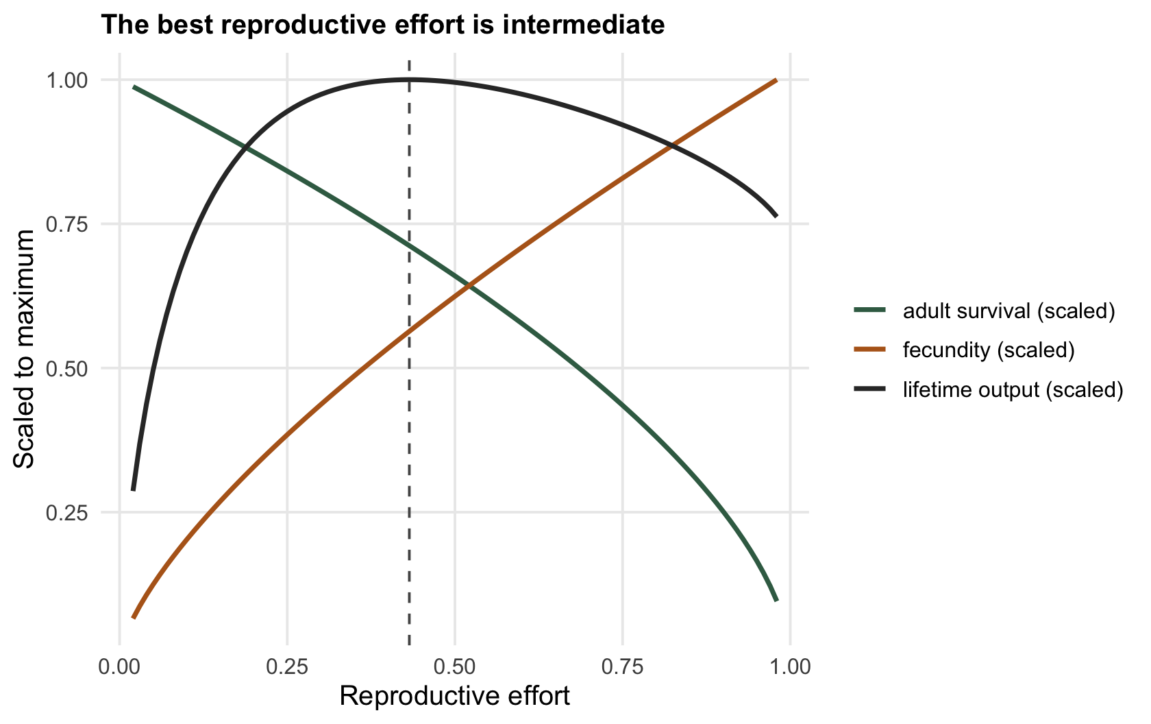
The best effort is intermediate, `r sprintf("%.2f", Estar)`, giving a lifetime output of `r sprintf("%.1f", R0star)`. Pour everything into a single reproductive event, effort of one, and lifetime output falls to `r sprintf("%.1f", R0_semel)`, because there is no second year. Holding back, breeding at moderate effort and surviving to breed again, beats going all in. This is iteroparity, repeated reproduction, winning over semelparity, a single fatal reproductive bout, and it wins here purely on the arithmetic of the trade-off.
```{r fig-tradeoff}
#| fig-cap: "The reproductive-effort trade-off. Fecundity (ochre) rises and adult survival (green) falls with effort; lifetime output (black) peaks at an intermediate effort, marked by the dashed line."
#| fig-alt: "Three curves against reproductive effort: fecundity rising, adult survival falling, and lifetime reproductive output peaking at an intermediate effort marked with a dashed vertical line."
Eg <- seq(0.02, 0.98, 0.01)
d <- rbind(data.frame(E = Eg, y = fec(Eg)/max(fec(Eg)), v = "fecundity (scaled)"),
           data.frame(E = Eg, y = sur(Eg)/smax,          v = "adult survival (scaled)"),
           data.frame(E = Eg, y = R0(Eg)/R0star,         v = "lifetime output (scaled)"))
ggplot(d, aes(E, y, colour = v)) +
  geom_line(linewidth = 1) +
  geom_vline(xintercept = Estar, colour = col_ref, linetype = "dashed") +
  scale_colour_manual(values = c("fecundity (scaled)" = col_fec, "adult survival (scaled)" = col_sur,
                                 "lifetime output (scaled)" = col_fit)) +
  labs(x = "Reproductive effort", y = "Scaled to maximum", colour = NULL,
       title = "The best reproductive effort is intermediate")
```
## Cole's paradox
If iteroparity is so good, why is any organism semelparous? Cole 1954 The Quarterly Review of Biology 29(2):103-137 sharpened the puzzle into a paradox. Compare an annual that breeds once and dies with a perennial that breeds every year forever. Cole's arithmetic said the annual needs only *one extra offspring* to match the perennial's long-run growth: an immortal perennial producing `b` offspring a year is matched by an annual producing `b + 1`. If one seed erases the whole advantage of living forever, why be perennial at all?
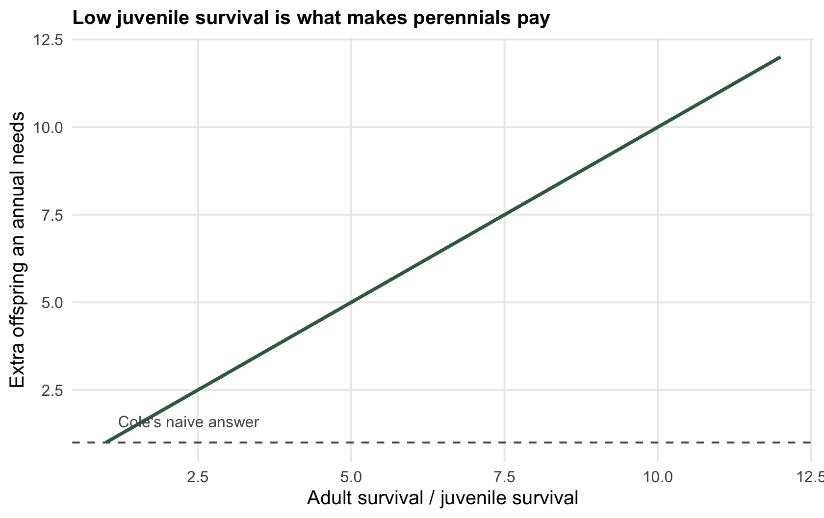
The resolution is that nobody lives forever, and juveniles and adults do not survive at the same rate (Charnov and Schaffer's correction). Put in realistic survivals and the "one extra offspring" becomes the ratio of adult to juvenile survival.
```{r cole}
juv <- 0.1; adult <- 0.8
c(cole_naive_extra = 1, corrected_extra = adult / juv)
```
With adult survival of `r sprintf("%.1f", adult)` and juvenile survival of `r sprintf("%.1f", juv)`, the annual needs `r sprintf("%.0f", cole_extra)` extra offspring, not one, to match the perennial. When juveniles die young and adults are tough, a perennial's surviving body is worth many risky seeds, and iteroparity is strongly favoured. The paradox dissolves once the survivals are honest.
```{r fig-cole}
#| fig-cap: "The extra offspring an annual needs to match a perennial, against the ratio of adult to juvenile survival. Cole's naive answer (one, dashed) holds only when the survivals are equal; low juvenile survival makes the true cost of being annual large."
#| fig-alt: "A rising straight line showing the extra offspring needed increasing with the adult-to-juvenile survival ratio, starting on the dashed line at one where the ratio is one and climbing well above it."
ra <- seq(1, 12, 0.1)
ggplot(data.frame(ratio = ra, extra = ra), aes(ratio, extra)) +
  geom_hline(yintercept = 1, colour = col_ref, linetype = "dashed") +
  geom_line(colour = col_sur, linewidth = 1) +
  annotate("text", x = 3, y = 1.5, label = "Cole's naive answer", hjust = 0, colour = col_ref, size = 3.4) +
  labs(x = "Adult survival / juvenile survival", y = "Extra offspring an annual needs",
       title = "Low juvenile survival is what makes perennials pay")
```
## What sets the optimum
Two things decide these answers, and both are assumptions worth stating. The first is the shape of the trade-off: change how steeply survival falls with effort and the optimal effort moves. The second is the currency. Here fitness was lifetime output, `R0`, which is right for a stationary population. In a growing one the right currency is the intrinsic rate `r`, which discounts late reproduction and can favour breeding early and hard, and in a variable one it is the geometric mean growth rate, which is where bet-hedging comes in. The [checking post](../checking-a-life-history-analysis/) shows how much the currency alone can move the optimum. The next two posts take the variable environment seriously: why fitness there is a geometric mean, and what that does to how much a plant should germinate.
## References
- Cole LC 1954. The Quarterly Review of Biology 29(2):103-137 (10.1086/400074).
- Stearns SC 1989. Functional Ecology 3(3):259-268 (10.2307/2389364).
- Charnov EL and Schaffer WM 1973. The American Naturalist 107(958):791-793 (10.1086/282877).
## Related tutorials
- [Bet-hedging and geometric mean fitness](../bet-hedging-and-geometric-mean-fitness/)
- [The optimal germination fraction](../optimal-germination-fraction/)
- [Checking a life-history analysis](../checking-a-life-history-analysis/)
- [Life tables and lambda](../life-tables-and-lambda/)