---
title: "Checking a life-history analysis"
description: "Three checks for a life-history study in R: matching the fitness currency, the acquisition-allocation trap that hides trade-offs, and detecting bet-hedging."
date: "2026-07-02 09:00"
categories: [ecology tutorial, R, life history, model diagnostics, evolutionary ecology]
image: thumbnail.png
image-alt: "A scatter of survival investment against reproductive investment in two overlapping clouds, each with its own fitted line: one sloping up, the other sloping down. The relationship is positive when acquisition varies and negative when allocation varies, hiding or revealing a trade-off."
---
```{r setup}
#| code-fold: true
#| code-summary: "Setup: packages, colours and plot theme"
#| results: hide
#| message: false
#| warning: false
knitr::opts_chunk$set(echo = TRUE, message = FALSE, warning = FALSE,
                      dev = "png", dpi = 120, fig.path = "figures/",
                      fig.width = 7, fig.height = 4.4)
library(ggplot2)
theme_te <- theme_minimal(base_size = 12) +
  theme(panel.background = element_rect(fill = "#f5f4ee", colour = NA),
        plot.background  = element_rect(fill = "#f5f4ee", colour = NA),
        panel.grid.minor = element_blank(),
        plot.title = element_text(face = "bold", size = 12))
theme_set(theme_te)
col_r0 <- "#3a6b52"; col_r <- "#b5651d"; col_ref <- "#555555"

## (a) currency
euler_r <- function(ages, m) uniroot(function(r) sum(m*exp(-r*ages)) - 1, c(-1, 5))$root
r_early <- euler_r(1, 6); r_late <- euler_r(3, 6)
fmax <- 6; smax <- 0.85; fec <- function(E) fmax*E^0.7; sur <- function(E) smax*(1-E)^0.6
R0 <- function(E) fec(E)/(1 - sur(E))
r_of <- function(E) { s <- sur(E); m <- fec(E); uniroot(function(r) m*sum(s^(0:80)*exp(-r*(1:81))) - 1, c(-1, 5))$root }
Es <- seq(0.05, 0.999, 0.001)
E_R0 <- Es[which.max(sapply(Es, R0))]; E_r <- Es[which.max(sapply(Es, r_of))]

## (b) acquisition-allocation
set.seed(406); n <- 400
demo <- function(sdA, sdP) {
  A <- pmax(rnorm(n, 10, sdA), 1); P <- plogis(rnorm(n, 0, sdP))
  data.frame(repro = P*A, surv = (1-P)*A)
}
d_acq <- demo(4, 0.3); d_all <- demo(1, 1.5)
r_acq <- cor(d_acq$repro, d_acq$surv); r_all <- cor(d_all$repro, d_all$surv)
```
Life-history theory turns natural selection into an optimisation problem, and optimisation problems have a way of giving confident wrong answers when the objective is mis-specified. Three checks catch the usual ways a life-history analysis misleads: the wrong fitness currency, a trade-off hidden by variation between individuals, and a bet-hedging signal that lives in the variance rather than the mean.
## Check 1: is the fitness currency right for the environment?
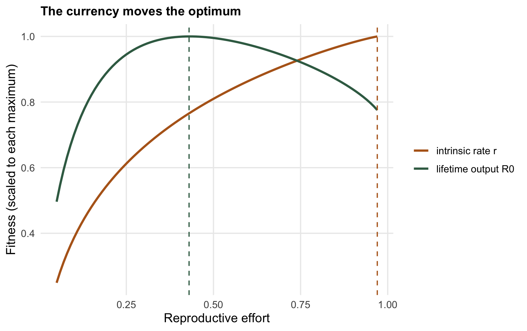
"Fitness" is not one number. In a stationary population it is lifetime reproductive output, `R0`. In a growing population it is the intrinsic rate of increase, `r`, which discounts offspring produced late because the population they join is already larger. In a fluctuating population it is the geometric mean growth rate. These currencies rank life histories differently, and the difference is not subtle.
```{r currency}
euler_r <- function(ages, m) uniroot(function(r) sum(m*exp(-r*ages)) - 1, c(-1, 5))$root
c(R0_both = 6, r_reproduce_early = euler_r(1, 6), r_reproduce_late = euler_r(3, 6))
```
Two schedules that produce the same six offspring over a lifetime have identical `R0`. But produced early, at age one, they buy an `r` of `r sprintf("%.2f", r_early)`; produced late, at age three, only `r sprintf("%.2f", r_late)`. Feed the reproductive-effort trade-off from the [first post](../life-history-trade-offs/) into each currency and the optimal effort itself moves: `R0` is maximised at an effort of `r sprintf("%.2f", E_R0)`, but `r` is maximised near `r sprintf("%.3f", E_r)`, pushing almost everything into reproducing now. Pick the currency that matches how the population is actually growing, or the optimum you compute is the answer to a different question.
```{r fig-currency}
#| fig-cap: "The same trade-off scored by two currencies, each scaled to its own maximum. Lifetime output (green) peaks at moderate effort; the intrinsic rate (ochre), which rewards early reproduction, peaks near maximal effort."
#| fig-alt: "Two scaled fitness curves against reproductive effort; the lifetime-output curve peaks at intermediate effort while the intrinsic-rate curve peaks near maximum effort."
dc <- rbind(data.frame(E = Es, y = sapply(Es, R0)/max(sapply(Es, R0)),   currency = "lifetime output R0"),
            data.frame(E = Es, y = sapply(Es, r_of)/max(sapply(Es, r_of)), currency = "intrinsic rate r"))
ggplot(dc, aes(E, y, colour = currency)) +
  geom_line(linewidth = 1) +
  geom_vline(xintercept = E_R0, colour = col_r0, linetype = "dashed") +
  geom_vline(xintercept = E_r, colour = col_r, linetype = "dashed") +
  scale_colour_manual(values = c("lifetime output R0" = col_r0, "intrinsic rate r" = col_r)) +
  labs(x = "Reproductive effort", y = "Fitness (scaled to each maximum)", colour = NULL,
       title = "The currency moves the optimum")
```
## Check 2: is the trade-off hidden by individual quality?
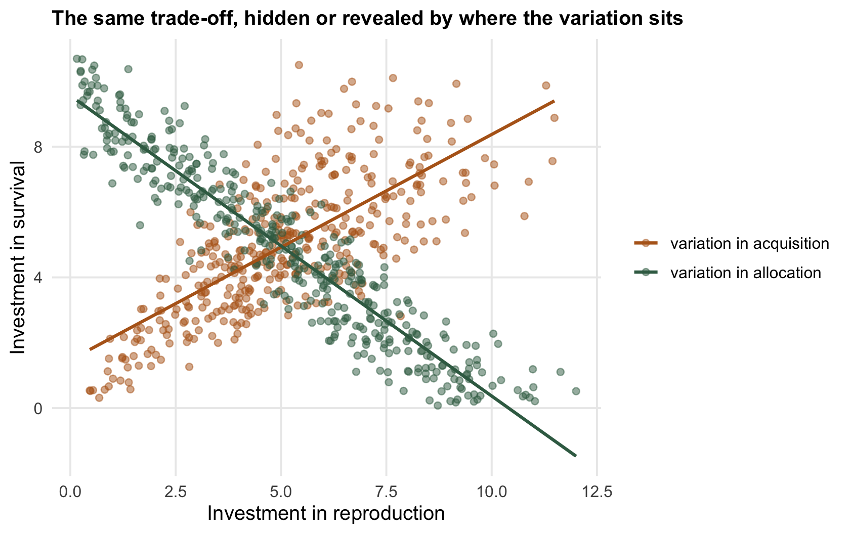
The core trade-offs, reproduction against survival, are trade-offs *within* an individual's budget: spend on one and less is left for the other. But we usually measure them *across* individuals, and individuals differ in how much they have to spend. A high-quality individual with a large budget can afford both high fecundity and high survival, while a poor one manages neither, so across a population the two can be *positively* correlated even though the allocation trade-off is strict. Van Noordwijk and de Jong 1986 The American Naturalist 128(1):137-142 made this precise: whether the trade-off shows depends on whether individuals vary more in acquisition or in allocation.
```{r acq-alloc}
set.seed(406); n <- 400
demo <- function(sdA, sdP) {
  A <- pmax(rnorm(n, 10, sdA), 1)          # resource acquisition (budget)
  P <- plogis(rnorm(n, 0, sdP))            # allocation fraction to reproduction (a strict trade-off)
  data.frame(repro = P*A, surv = (1-P)*A)
}
d_acq <- demo(4, 0.3)                      # individuals vary mostly in budget
d_all <- demo(1, 1.5)                      # individuals vary mostly in split
c(variation_in_acquisition = cor(d_acq$repro, d_acq$surv),
  variation_in_allocation  = cor(d_all$repro, d_all$surv))
```
When individuals vary mostly in acquisition, the observed correlation between reproduction and survival investment is `r sprintf("%+.2f", r_acq)`, positive: the data say "more reproduction goes with more survival", the opposite of a trade-off. When they vary mostly in allocation, the correlation is `r sprintf("%+.2f", r_all)`, the real negative trade-off. The underlying allocation rule is identical in both; only the source of variation differs. A raw phenotypic correlation across individuals is therefore no test of a trade-off. What tests it is manipulation, add offspring to a brood experimentally and measure the survival cost, or a design that holds acquisition constant.
```{r fig-acq}
#| fig-cap: "Reproduction against survival investment for the same allocation trade-off. When acquisition varies (ochre) the cloud slopes up and hides the trade-off; when allocation varies (green) it slopes down and reveals it."
#| fig-alt: "Two scatter clouds of reproduction against survival investment; the ochre cloud from variable acquisition slopes upward, the green cloud from variable allocation slopes downward."
dd <- rbind(cbind(d_acq, case = "variation in acquisition"), cbind(d_all, case = "variation in allocation"))
ggplot(dd, aes(repro, surv, colour = case)) +
  geom_point(size = 1.6, alpha = 0.5) +
  geom_smooth(method = "lm", se = FALSE, linewidth = 0.9) +
  scale_colour_manual(values = c("variation in acquisition" = col_r, "variation in allocation" = col_r0)) +
  labs(x = "Investment in reproduction", y = "Investment in survival", colour = NULL,
       title = "The same trade-off, hidden or revealed by where the variation sits")
```
## Check 3: is the signal in the mean or the variance?
Bet-hedging is invisible to the usual analysis because it does not optimise the mean. A bet-hedging phenotype deliberately accepts a lower arithmetic-mean fitness to cut variance, so measured against the mean it looks *suboptimal*, and an analysis that scores strategies by average success will reject it. Detecting it requires the thing that is hardest to measure: variance in fitness across generations, which needs long runs of data on marked individuals or genotypes, not a single well-sampled year. This is why the empirical evidence for bet-hedging remains thin despite strong theory, and why claims of it demand a demonstration that the variance, not just the mean, is doing the work (Simons 2011 Proceedings of the Royal Society B 278(1712):1601-1609).
## The theory is only as good as its objective
These three checks share a theme: the machinery of life-history optimisation is sound, and the danger is all in what you feed it. The wrong currency, a correlation mistaken for a trade-off, or a mean where the variance is the point will each produce a clean, confident, wrong optimum. State the fitness measure and justify it, test trade-offs by manipulation rather than correlation, and when variance is the hypothesis, measure variance. The optimum is only as trustworthy as the objective it maximised.
## References
- Simons AM 2011. Proceedings of the Royal Society B 278(1712):1601-1609 (10.1098/rspb.2011.0176).
- van Noordwijk AJ, de Jong G 1986. The American Naturalist 128(1):137-142 (10.1086/284547).
## Related tutorials
- [Life-history trade-offs in R](../life-history-trade-offs/)
- [Bet-hedging and geometric mean fitness](../bet-hedging-and-geometric-mean-fitness/)
- [The optimal germination fraction](../optimal-germination-fraction/)
- [The life-table response experiment](../life-table-response-experiment/)