---
title: "The optimal germination fraction"
description: "Delayed germination as bet-hedging in R: Cohen's model of the optimal fraction of seeds to germinate in a variable environment, and why it is less than one."
date: "2026-07-01 15:00"
categories: [ecology tutorial, R, life history, evolutionary ecology, plant ecology]
image: thumbnail.png
image-alt: "Long-run growth against germination fraction for several bad-year frequencies, each peaking at a fraction below one."
---
```{r setup}
#| code-fold: true
#| code-summary: "Setup: packages, colours and plot theme"
#| results: hide
#| message: false
#| warning: false
knitr::opts_chunk$set(echo = TRUE, message = FALSE, warning = FALSE,
                      dev = "png", dpi = 120, fig.path = "figures/",
                      fig.width = 7, fig.height = 4.4)
library(ggplot2)
theme_te <- theme_minimal(base_size = 12) +
  theme(panel.background = element_rect(fill = "#f5f4ee", colour = NA),
        plot.background  = element_rect(fill = "#f5f4ee", colour = NA),
        panel.grid.minor = element_blank(),
        plot.title = element_text(face = "bold", size = 12))
theme_set(theme_te)
pal <- c("#3a6b52", "#7a8b5a", "#b5651d"); col_ref <- "#555555"

s <- 0.9; Ygood <- 8
gm_growth <- function(G, pbad) exp(pbad*log((1-G)*s + G*0) + (1-pbad)*log((1-G)*s + G*Ygood))
Gs <- seq(0.001, 1, 0.001)
Gstar <- function(pbad) Gs[which.max(sapply(Gs, gm_growth, pbad = pbad))]
g_star <- sapply(c(0.1, 0.3, 0.5), Gstar)
```
An annual plant faces a gamble every spring. Germinate, and if the year is good you reproduce, but if it is a drought you die before setting seed. The obvious strategy, germinate every seed and get on with it, is a trap in a variable climate, because a single bad year kills the entire cohort at once. Cohen 1966 Journal of Theoretical Biology 12(1):119-129 showed that the right answer is to hold some seeds back, and worked out exactly how many. It is one of the cleanest results in evolutionary ecology, and it is a few lines of R.
## The seed-bank model
Track a population of seeds. Each year a fraction `G` germinates and the rest, `1 - G`, stay dormant in the soil and survive to next year with probability `s`. A germinated seed in a good year yields `Y` new seeds; in a bad year it yields nothing and is lost. The seed population multiplies each year by
$$\lambda_t = (1 - G)\,s + G\,Y_t,$$
the dormant survivors plus the germinated seeds' yield. Because the population multiplies year on year, its long-run growth is the geometric mean of these annual factors, not the arithmetic mean, exactly the lesson of [the previous post](../bet-hedging-and-geometric-mean-fitness/).
```{r model}
s <- 0.9; Ygood <- 8                                   # dormant survival; good-year yield
gm_growth <- function(G, pbad) {                       # long-run (geometric-mean) growth
  exp(pbad*log((1-G)*s + G*0) + (1-pbad)*log((1-G)*s + G*Ygood))
}
c(germinate_all = gm_growth(1, pbad = 0.3), germinate_half = gm_growth(0.5, pbad = 0.3))
```
Germinating everything, `G = 1`, is fatal in a variable climate: in any bad year the factor is $(1 - 1)s + 1 \times 0 = 0$, and one zero in the product drags the whole geometric mean to zero. The population is one drought from extinction. Holding half the seeds back keeps a reserve that carries the lineage through the bad year.
## The optimum is less than one
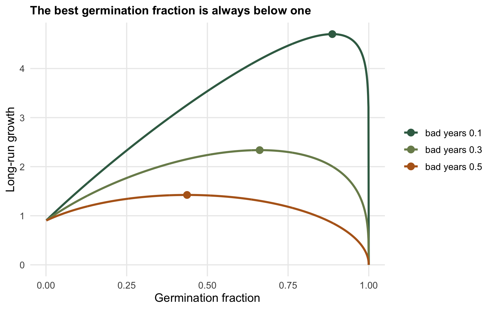
Sweep the germination fraction and find the value that maximises long-run growth, for climates that differ in how often the bad year strikes.
```{r optima}
Gs <- seq(0.001, 1, 0.001)
Gstar <- function(pbad) Gs[which.max(sapply(Gs, gm_growth, pbad = pbad))]
sapply(c(0.1, 0.3, 0.5), Gstar)                        # optimal G at three bad-year frequencies
```
When bad years are rare, one in ten, the plant should germinate most of its seeds, `r sprintf("%.2f", g_star[1])`; when they are common, one in two, it should germinate less than half, `r sprintf("%.2f", g_star[3])`, and keep the rest safe underground. In every case the optimum is below one: some fraction of seeds should always wait. The riskier the climate, the deeper the plant should bank. This is diversified bet-hedging spread across time, the seeds of one year hedged over several future years, and it explains why so many desert annuals and weeds carry persistent seed banks that a purely arithmetic accounting would call wasteful.
```{r fig-optimum}
#| fig-cap: "Long-run growth against germination fraction, for three climates. Each curve peaks at a fraction below one (marked), and the peak moves left as bad years get more frequent. Germinating everything collapses growth to zero."
#| fig-alt: "Three humped curves of long-run growth against germination fraction, each peaking below a fraction of one, with the peak shifting left as the bad-year frequency rises."
curves <- do.call(rbind, lapply(c(0.1, 0.3, 0.5), function(pb)
  data.frame(G = Gs, growth = sapply(Gs, gm_growth, pbad = pb), pbad = paste0("bad years ", pb))))
pts <- data.frame(G = g_star, pbad = paste0("bad years ", c(0.1, 0.3, 0.5)))
pts$growth <- mapply(function(g, pb) gm_growth(g, pb), pts$G, c(0.1, 0.3, 0.5))
ggplot(curves, aes(G, growth, colour = pbad)) +
  geom_line(linewidth = 1) +
  geom_point(data = pts, aes(G, growth, colour = pbad), size = 3) +
  scale_colour_manual(values = setNames(pal, paste0("bad years ", c(0.1, 0.3, 0.5)))) +
  labs(x = "Germination fraction", y = "Long-run growth", colour = NULL,
       title = "The best germination fraction is always below one")
```
## How the bank tracks the risk
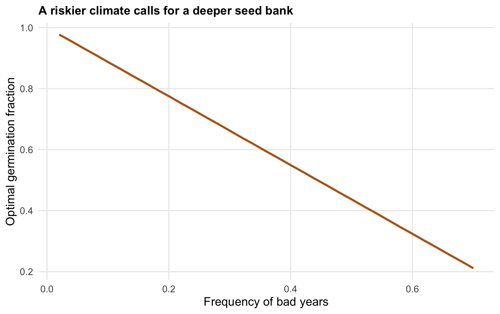
Trace the optimum across the whole range of climates and the relationship is smooth and monotone: every increase in the frequency of bad years lowers the fraction a plant should germinate.
```{r fig-gstar}
#| fig-cap: "Optimal germination fraction against the frequency of bad years. It falls steadily from near one in a benign climate toward a cautious fraction as bad years become common."
#| fig-alt: "A declining curve of optimal germination fraction against the frequency of bad years, from high in benign climates to low in risky ones."
pb <- seq(0.02, 0.7, 0.02)
dg <- data.frame(pbad = pb, Gstar = sapply(pb, Gstar))
ggplot(dg, aes(pbad, Gstar)) +
  geom_line(colour = "#b5651d", linewidth = 1) +
  labs(x = "Frequency of bad years", y = "Optimal germination fraction",
       title = "A riskier climate calls for a deeper seed bank")
```
## The assumptions that set the number
The exact optimum depends on things the model fixed and a real plant would not. Dormant seeds do not survive perfectly; raise their death rate in the soil and banking becomes less attractive, pushing the optimal fraction back up. More importantly, the model assumes bad years are unpredictable. If a plant can read a cue, autumn rainfall, temperature, that forecasts the coming season, it should germinate in response to the cue rather than hedge blindly, and predictive germination replaces bet-hedging to the extent the cue is reliable. Density dependence, seed predation, and a spread of yields rather than a clean good-or-bad split all shift the number too. The dependable prediction is not the exact fraction but its direction: unpredictable risk selects for delayed germination, and more risk selects for more of it. Whether a real seed bank is bet-hedging or something else is a question the [checking post](../checking-a-life-history-analysis/) treats with the caution it needs.
## References
- Cohen D 1966. Journal of Theoretical Biology 12(1):119-129 (10.1016/0022-5193(66)90188-3).
- Philippi T, Seger J 1989. Trends in Ecology and Evolution 4(2):41-44 (10.1016/0169-5347(89)90138-9).
## Related tutorials
- [Bet-hedging and geometric mean fitness](../bet-hedging-and-geometric-mean-fitness/)
- [Life-history trade-offs in R](../life-history-trade-offs/)
- [Checking a life-history analysis](../checking-a-life-history-analysis/)
- [Annual plant competition models](../annual-plant-competition-models/)