---
title: "Bet-hedging and geometric mean fitness"
description: "Why fitness in a variable environment is the geometric mean, not the arithmetic: bet-hedging in R, and how a lower-mean, steadier strategy wins the long run."
date: "2026-07-01 14:00"
date-modified: "2026-10-07"
categories: [ecology tutorial, R, life history, evolutionary ecology, bet-hedging]
image: thumbnail.png
image-alt: "Many simulated lineage trajectories: a risky strategy spreading and mostly crashing, a steady strategy climbing together on a log scale."
---
*Corrected 7 October 2026: the section on the variance tax said that once the geometric mean drops below one the lineage is doomed on average; it now says the typical lineage is doomed even though the average year is still above one.*
```{r setup}
#| code-fold: true
#| code-summary: "Setup: packages, colours and plot theme"
#| results: hide
#| message: false
#| warning: false
knitr::opts_chunk$set(echo = TRUE, message = FALSE, warning = FALSE,
                      dev = "png", dpi = 120, fig.path = "figures/",
                      fig.width = 7, fig.height = 4.4)
library(ggplot2)
theme_te <- theme_minimal(base_size = 12) +
  theme(panel.background = element_rect(fill = "#f5f4ee", colour = NA),
        plot.background  = element_rect(fill = "#f5f4ee", colour = NA),
        panel.grid.minor = element_blank(),
        plot.title = element_text(face = "bold", size = 12))
theme_set(theme_te)
col_risky <- "#b5651d"; col_steady <- "#3a6b52"; col_ref <- "#555555"

A_good <- 2.0; A_bad <- 0.4; p <- 0.5; B <- 1.1
am_A <- p*A_good + (1-p)*A_bad
gm_A <- A_good^p * A_bad^(1-p)
years <- 40
set.seed(403)
run <- function(good, bad, pg, reps) {
  M <- matrix(1, reps, years + 1)
  for (t in 2:(years + 1)) M[, t] <- M[, t-1] * ifelse(runif(reps) < pg, good, bad)
  M
}
RA <- run(A_good, A_bad, p, 2000); RB <- run(B, B, p, 2000)
medA <- median(RA[, years+1]); medB <- median(RB[, years+1])
ext_A <- 100 * mean(RA[, years+1] < 0.01)
```
The most common mistake in thinking about fitness in a variable environment is to average the wrong way. A strategy that does brilliantly in good years and terribly in bad ones can have a higher *average* yearly output than a steady rival and still lose, decisively, over the long run. The reason is that a lineage multiplies its numbers year on year, and what governs a product is the geometric mean, not the arithmetic one. Everything about bet-hedging follows from that single fact (Philippi and Seger 1989 Trends in Ecology and Evolution 4(2):41-44).
## Two ways to average
Take a risky strategy that doubles in a good year and shrinks to `r sprintf("%.1f", A_bad)` in a bad one, each with even odds, against a steady strategy that grows by a flat `r sprintf("%.1f", B)` every year regardless.
```{r means}
A_good <- 2.0; A_bad <- 0.4; p <- 0.5; B <- 1.1
c(risky_arithmetic = p*A_good + (1-p)*A_bad,
  risky_geometric  = A_good^p * A_bad^(1-p),
  steady_both      = B)
```
The risky strategy has the higher arithmetic mean, `r sprintf("%.2f", am_A)` against `r sprintf("%.2f", B)`: on an average year it grows faster. But its geometric mean is `r sprintf("%.3f", gm_A)`, below one, which means that compounded over years it *shrinks*. The steady strategy's geometric mean is its arithmetic mean, `r sprintf("%.2f", B)`, and it grows. Judged by the average year the risky strategy looks better; judged by the long run it goes extinct while the steady one thrives.
## Watch it happen
Averages can feel abstract, so simulate many independent lineages of each strategy over `r sprintf("%.0f", years)` years and look at where they end up.
```{r simulate}
years <- 40
set.seed(403)
step <- function(N, good, bad, pg) N * ifelse(runif(length(N)) < pg, good, bad)
sim  <- function(good, bad, pg, reps) { N <- rep(1, reps); for (t in 1:years) N <- step(N, good, bad, pg); N }
final_A <- sim(A_good, A_bad, p, 2000); final_B <- sim(B, B, p, 2000)
c(median_risky = median(final_A), median_steady = median(final_B),
  risky_percent_extinct = 100 * mean(final_A < 0.01))
```
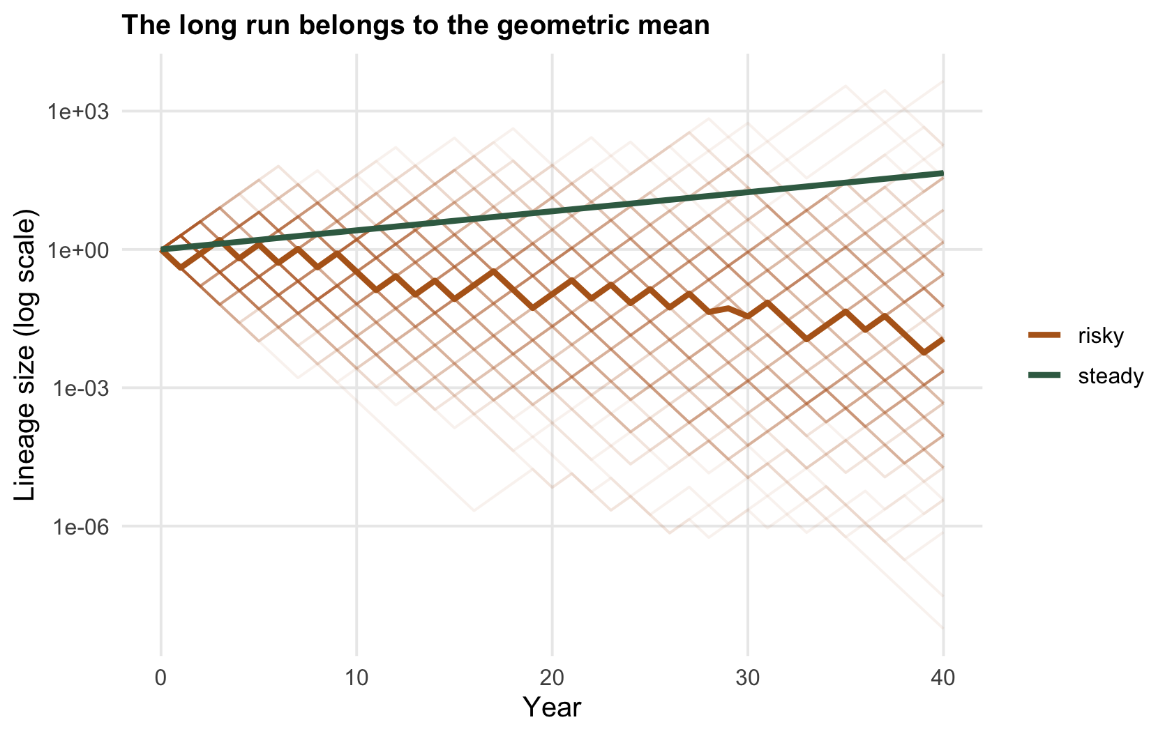
After forty years the median steady lineage has grown to about `r sprintf("%.0f", medB)` times its start; the median risky lineage has collapsed to `r sprintf("%.3f", medA)`, a hundredth of where it began, and `r sprintf("%.0f", ext_A)` per cent of risky lineages are effectively extinct. A few risky lineages get a lucky run of good years and shoot up, which is what props up the arithmetic mean, but they are rare, and betting a lineage on being one of them is a losing strategy.
```{r fig-traj}
#| fig-cap: "Simulated lineages on a log scale. The steady strategy (green) climbs together; the risky one (ochre) fans out, a few soaring but most sinking. Thick lines are medians."
#| fig-alt: "Many faint trajectories on a log scale; green steady lineages rise along one shared line while ochre risky lineages spread widely, most declining below the start."
idx <- 1:120
tr <- rbind(
  do.call(rbind, lapply(idx, function(i) data.frame(t = 0:years, N = RA[i, ], grp = "risky", id = i))),
  do.call(rbind, lapply(idx, function(i) data.frame(t = 0:years, N = RB[i, ], grp = "steady", id = i))))
med <- rbind(data.frame(t = 0:years, N = apply(RA, 2, median), grp = "risky"),
             data.frame(t = 0:years, N = apply(RB, 2, median), grp = "steady"))
ggplot(tr, aes(t, N, group = interaction(grp, id), colour = grp)) +
  geom_line(alpha = 0.08) +
  geom_line(data = med, aes(t, N, group = grp, colour = grp), linewidth = 1.2) +
  scale_y_log10() +
  scale_colour_manual(values = c("risky" = col_risky, "steady" = col_steady)) +
  labs(x = "Year", y = "Lineage size (log scale)", colour = NULL,
       title = "The long run belongs to the geometric mean")
```
## Variance is a tax on fitness
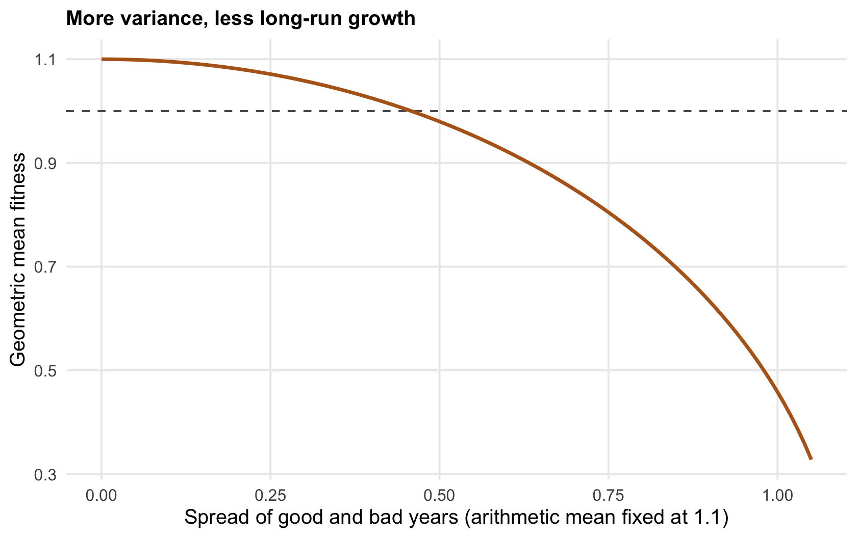
Bet-hedging is the strategy of trading away some arithmetic mean to cut variance, because cutting variance raises the geometric mean. How steep is that trade? Hold the arithmetic mean fixed and widen the spread of good and bad years around it: the geometric mean falls, and past a point it drops below one and the typical lineage is doomed, even though the average year is still above one.
```{r variance-tax}
gm_fixed_mean <- function(delta, m = 1.1) sqrt((m + delta) * (m - delta))  # same arithmetic mean m
sapply(c(0, 0.3, 0.6, 0.9), gm_fixed_mean)
```
At the same arithmetic mean of `r sprintf("%.1f", 1.1)`, a spread of zero leaves the geometric mean at `r sprintf("%.2f", 1.1)`; widen the good and bad years to plus or minus `r sprintf("%.1f", 0.9)` and the geometric mean falls to `r sprintf("%.2f", sqrt((1.1+0.9)*(1.1-0.9)))`. The approximation is worth remembering: the geometric mean is roughly the arithmetic mean minus the variance divided by twice the mean. Variance is subtracted from fitness directly, which is why a strategy that lowers variance, even at some cost to the average, can win.
```{r fig-tax}
#| fig-cap: "The variance tax. With the arithmetic mean fixed, wider year-to-year variation lowers the geometric mean; past the dashed line the lineage shrinks despite an above-one average year."
#| fig-alt: "A curve of geometric mean falling as the spread between good and bad years widens, crossing below one at large spreads while the arithmetic mean stays fixed."
dl <- data.frame(delta = seq(0, 1.05, 0.01)); dl$gm <- gm_fixed_mean(dl$delta)
ggplot(dl, aes(delta, gm)) +
  geom_hline(yintercept = 1, colour = col_ref, linetype = "dashed") +
  geom_line(colour = col_risky, linewidth = 1) +
  labs(x = "Spread of good and bad years (arithmetic mean fixed at 1.1)", y = "Geometric mean fitness",
       title = "More variance, less long-run growth")
```
## What bet-hedging is, and is not
Two clarifications keep this from being mis-applied. First, the variance that matters is the kind shared across the whole population in a given year, a good or bad year for everyone, because that is what erodes the lineage's geometric mean. Variation that is independent among individuals mostly averages out and does not select for hedging. Second, there are two ways to hedge: be conservative, adopt a lower-variance phenotype outright, or diversify, spread the bet across many offspring or many years so that some always land in a good year. The classic example of diversifying in time is a plant that declines to germinate all its seeds at once, the subject of the [next post](../optimal-germination-fraction/). Detecting either kind in real data is genuinely hard, because it requires measuring variance in fitness across generations rather than the mean, which the [checking post](../checking-a-life-history-analysis/) takes up (Simons 2011 Proceedings of the Royal Society B 278(1712):1601-1609).
## References
- Philippi T, Seger J 1989. Trends in Ecology and Evolution 4(2):41-44 (10.1016/0169-5347(89)90138-9).
- Simons AM 2011. Proceedings of the Royal Society B 278(1712):1601-1609 (10.1098/rspb.2011.0176).
## Related tutorials
- [Combining species trends into one index](../a-multi-species-index-and-its-arithmetic/)
- [The optimal germination fraction](../optimal-germination-fraction/)
- [Checking a life-history analysis](../checking-a-life-history-analysis/)
- [Stochastic population growth](../stochastic-population-growth/)